dsp.LMSFilter
Compute output, error, and weights of least mean squares (LMS) adaptive filter
Description
The dsp.LMSFilter
System object™ implements an adaptive finite impulse response (FIR) filter that converges an
input signal to the desired signal using one of the following algorithms:
LMS
Normalized LMS
Sign-Data LMS
Sign-Error LMS
Sign-Sign LMS
For more details on each of these methods, see Algorithms.
The filter adapts its weights until the error between the primary input signal and the
desired signal is minimal. The mean square of this error (MSE) is computed using the msesim function. The
predicted version of the MSE is determined using a Wiener filter in the msepred function.
The maxstep function
computes the maximum adaptation step size, which controls the speed of convergence.
For an overview of the adaptive filter methodology, and the most common applications the adaptive filters are used in, see Overview of Adaptive Filters and Applications.
To filter a signal using an adaptive FIR filter:
Create the
dsp.LMSFilterobject and set its properties.Call the object with arguments, as if it were a function.
To learn more about how System objects work, see What Are System Objects?
This object supports C/C++ code generation and SIMD code generation under certain conditions. For more information, see Code Generation.
Creation
Description
lms = dsp.LMSFilterlms, that computes the filtered output, filter
error, and the filter weights for a given input and a desired signal using the least mean
squares (LMS) algorithm.
lms = dsp.LMSFilter(
returns an LMS filter object with each specified property set to the specified value.
Enclose each property name in single quotes. You can use this syntax with the previous
input argument.PropertyName=Value)
Properties
Unless otherwise indicated, properties are nontunable, which means you cannot change their
values after calling the object. Objects lock when you call them, and the
release function unlocks them.
If a property is tunable, you can change its value at any time.
For more information on changing property values, see System Design in MATLAB Using System Objects.
Method to calculate filter weights, specified as one of the following:
'LMS'–– Solves the Wiener-Hopf equation and finds the filter coefficients for an adaptive filter.'Normalized LMS'–– Normalized variation of the LMS algorithm.'Sign-Data LMS'–– Correction to the filter weights at each iteration depends on the sign of the inputx.'Sign-Error LMS'–– Correction applied to the current filter weights for each successive iteration depends on the sign of the error,err.'Sign-Sign LMS'–– Correction applied to the current filter weights for each successive iteration depends on both the sign ofxand the sign oferr.
For more details on the algorithms, see Algorithms.
Length of the FIR filter weights vector, specified as a positive integer.
Example: 64
Example: 16
Data Types: single | double | int8 | int16 | int32 | int64 | uint8 | uint16 | uint32 | uint64
Method to specify the adaptation step size, specified as one of the following:
'Property'–– The property StepSize specifies the size of each adaptation step.'Input port'–– Specify the adaptation step size as one of the inputs to the object.
Adaptation step size factor, specified as a non-negative scalar. For convergence of the normalized LMS method, the step size must be greater than 0 and less than 2.
A small step size ensures a small steady state error between the output y and the desired signal
d. If the step size is
small, the convergence speed of the filter decreases. To improve the convergence speed,
increase the step size. Note that if the step size is large, the filter can become
unstable. To compute the maximum step size the filter can accept without becoming
unstable, use the maxstep
function.
Tunable: Yes
Dependencies
This property applies when you set StepSizeSource to
'Property'.
Data Types: single | double | int8 | int16 | int32 | int64 | uint8 | uint16 | uint32 | uint64
Leakage factor used when implementing the leaky LMS method, specified as a scalar in
the range [0 1]. When the value equals 1, there is no leakage in the
adapting method. When the value is less than 1, the filter implements a leaky LMS
method.
Example: 0.5
Tunable: Yes
Data Types: single | double | int8 | int16 | int32 | int64 | uint8 | uint16 | uint32 | uint64
Initial conditions of filter weights, specified as a scalar or a vector of length equal to the value of the Length property. When the input is real, the value of this property must be real.
Example: 0
Example: [1 3 1 2 7 8 9 0 2 2 8 2]
Data Types: single | double | int8 | int16 | int32 | int64 | uint8 | uint16 | uint32 | uint64
Complex Number Support: Yes
Flag to adapt filter weights, specified as one of the following:
false–– The object continuously updates the filter weights.true–– An adaptation control input is provided to the object when you call its algorithm. If the value of this input is non-zero, the object continuously updates the filter weights. If the value of this input is zero, the filter weights remain at their current value.
Flag to reset filter weights, specified as one of the following:
false–– The object does not reset weights.true–– A reset control input is provided to the object when you call its algorithm. This setting enables the WeightsResetCondition property. The object resets the filter weights based on the values of theWeightsResetConditionproperty and the reset input provided to the object algorithm.
Event that triggers the reset of the filter weights, specified as one of the following. The object resets the filter weights whenever a reset event is detected in its reset input.
'Non-zero'–– Triggers a reset operation at each sample, when the reset input is not zero.'Rising edge'–– Triggers a reset operation when the reset input does one of the following:Rises from a negative value to either a positive value or zero.
Rises from zero to a positive value, where the rise is not a continuation of a rise from a negative value to zero.

'Falling edge'–– Triggers a reset operation when the reset input does one of the following:Falls from a positive value to a negative value or zero.
Falls from zero to a negative value, where the fall is not a continuation of a fall from a positive value to zero.

'Either edge'–– Triggers a reset operation when the reset input is a rising edge or a falling edge.
The object resets the filter weights based on the value of this property and the
reset input r provided to the object algorithm.
Dependencies
This property applies when you set the WeightsResetInputPort property to
true.
Method to output adapted filter weights, specified as one of the following:
'Last'(default) — The object returns a column vector of weights corresponding to the last sample of the data frame. The length of the weights vector is the value given by the Length property.'All'— The object returns a FrameLength-by-Length matrix of weights. The matrix corresponds to the full sample-by-sample history of weights for all FrameLength samples of the input values. Each row in the matrix corresponds to a set of LMS filter weights calculated for the corresponding input sample.'None'— This setting disables the weights output.
Fixed-Point Properties
Specify the rounding mode for fixed-point operations. For more details, see rounding mode.
Overflow action for fixed-point operations, specified as one of the following:
'Wrap'–– The object wraps the result of its fixed-point operations.'Saturate'–– The object saturates the result of its fixed-point operations.
For more details on overflow actions, see overflow mode for fixed-point operations.
Step size word length and fraction length settings, specified as one of the following:
'Same word length as first input'–– The object specifies the word length of step size to be the same as that of the first input. The fraction length is computed to get the best possible precision.'Custom'–– The step size data type is specified as a custom numeric type through the CustomStepSizeDataType property.
For more information on the step size data type this object uses, see the Fixed Point section.
Word and fraction lengths of the step size, specified as an autosigned numeric type with a word length of 16 and a fraction length of 15.
Example: numerictype([],32)
Dependencies
This property applies under the following conditions:
StepSizeSource property set to
'Property'and StepSizeDataType set to'Custom'.StepSizeSourceproperty set to'Input port'.
Leakage factor word length and fraction length settings, specified as one of the following:
'Same word length as first input'–– The object specifies the word length of leakage factor to be the same as that of the first input. The fraction length is computed to get the best possible precision.'Custom'–– The leakage factor data type is specified as a custom numeric type through the CustomLeakageFactorDataType property.
For more information on the leakage factor data type this object uses, see the Fixed Point section.
Word and fraction lengths of the leakage factor, specified as an autosigned numeric type with a word length of 16 and a fraction length of 15.
Example: numerictype([],32)
Dependencies
This property applies when you set the LeakageFactorDataType property to
'Custom'.
Weights word length and fraction length settings, specified as one of the following:
'Same as first input'–– The object specifies the data type of the filter weights to be the same as that of the first input.'Custom'–– The data type of filter weights is specified as a custom numeric type through the CustomWeightsDataType property.
For more information on the filter weights data type this object uses, see the Fixed Point section.
Word and fraction lengths of the filter weights, specified as an autosigned numeric type with a word length of 16 and a fraction length of 15.
Example: numerictype([],32,20)
Dependencies
This property applies when you set the WeightsDataType property to
'Custom'.
Energy product word length and fraction length settings, specified as one of the following:
'Same as first input'–– The object specifies the data type of the energy product to be the same as that of the first input.'Custom'–– The data type of the energy product is specified as a custom numeric type through the CustomEnergyProductDataType property.
For more information on the energy product data type this object uses, see the Fixed Point section.
Dependencies
This property applies when you set the Method property to 'Normalized
LMS'.
Word and fraction lengths of the energy product, specified as an autosigned numeric type with a word length of 32 and a fraction length of 20.
Dependencies
This property applies when you set the Method property to 'Normalized
LMS' and EnergyProductDataType property to
'Custom'.
Energy accumulator word length and fraction length settings, specified as one of the following:
'Same as first input'–– The object specifies the data type of the energy accumulator to be the same as that of the first input.'Custom'–– The data type of the energy accumulator is specified as a custom numeric type through the CustomEnergyAccumulatorDataType property.
For more information on the energy accumulator data type this object uses, see the Fixed Point section.
Dependencies
This property applies when you set the Method property to 'Normalized
LMS'.
Word and fraction lengths of the energy accumulator, specified as an autosigned numeric type with a word length of 32 and a fraction length of 20.
Dependencies
This property applies when you set the Method property to 'Normalized
LMS' and EnergyAccumulatorDataType property to
'Custom'.
Convolution product word length and fraction length settings, specified as one of the following:
'Same as first input'–– The object specifies the data type of the convolution product to be the same as that of the first input.'Custom'–– The data type of the convolution product is specified as a custom numeric type through the CustomConvolutionProductDataType property.
For more information on the convolution product data type this object uses, see the Fixed Point section.
Word and fraction lengths of the convolution product, specified as an autosigned numeric type with a word length of 32 and a fraction length of 20.
Dependencies
This property applies when you set the ConvolutionProductDataType property to
'Custom'.
Convolution accumulator word length and fraction length settings, specified as one of the following:
'Same as first input'–– The object specifies the data type of the convolution accumulator to be the same as that of the first input.'Custom'–– The data type of the convolution accumulator is specified as a custom numeric type through the CustomConvolutionAccumulatorDataType property.
For more information on the convolution accumulator data type this object uses, see the Fixed Point section.
Word and fraction lengths of the convolution accumulator, specified as an autosigned numeric type with a word length of 32 and a fraction length of 20.
Dependencies
This property applies when you set the ConvolutionAccumulatorDataType property to
'Custom'.
Step size error product word length and fraction length settings, specified as one of the following:
'Same as first input'–– The object specifies the data type of the step size error product to be the same as that of the first input.'Custom'–– The data type of the step size error product is specified as a custom numeric type through the CustomStepSizeErrorProductDataType property.
For more information on the step size error product data type this object uses, see the Fixed Point section.
Word and fraction lengths of the step size error product, specified as an autosigned numeric type with a word length of 32 and a fraction length of 20.
Dependencies
This property applies when you set the StepSizeErrorProductDataType property to
'Custom'.
Word and fraction length settings of the filter weights update product, specified as one of the following:
'Same as first input'–– The object specifies the data type of the filter weights update product to be the same as that of the first input.'Custom'–– The data type of the filter weights update product is specified as a custom numeric type through the CustomWeightsUpdateProductDataType property.
For more information on the filter weights update product data type this object uses, see the Fixed Point section.
Word and fraction lengths of the filter weights update product, specified as an autosigned numeric type with a word length of 32 and a fraction length of 20.
Dependencies
This property applies when you set the WeightsUpdateProductDataType property to
'Custom'.
Quotient word length and fraction length settings, specified as one of the following:
'Same as first input'–– The object specifies the quotient data type to be the same as that of the first input.'Custom'–– The quotient data type is specified as a custom numeric type through the CustomQuotientDataType property.
For more information on the quotient data type this object uses, see the Fixed Point section.
Dependencies
This property applies when you set the Method property to 'Normalized
LMS'.
Word and fraction lengths of the filter weights update product, specified as an autosigned numeric type with a word length of 32 and a fraction length of 20.
Dependencies
This property applies when you set the Method property to 'Normalized
LMS' and QuotientDataType property to
'Custom'.
Usage
Syntax
Description
[
filters the input signal, y,err,wts] = lms(x,d)x, using d as the
desired signal, and returns the filtered output in y, the filter
error in err, and the estimated filter weights in
wts. The LMS filter object estimates the filter weights needed to
minimize the error between the output signal and the desired signal.
[
filters the input signal, y,err] = lms(x,d)x, using d as the
desired signal, and returns the filtered output in y and the filter
error in err when the WeightsOutput property is set to
'None'.
[___] = lms(
filters the input signal, x,d,mu)x, using d as the
desired signal and mu as the step size, when the StepSizeSource property is set to 'Input
port'. These inputs can be used with either of the previous sets of
outputs.
[___] = lms(
filters the input signal, x,d,a)x, using d as the
desired signal and a as the adaptation control when the AdaptInputPort property is set to
true. When a is nonzero, the System object continuously updates the filter weights. When a is
zero, the filter weights remain constant.
[___] = lms(
filters the input signal, x,d,r)x, using d as the
desired signal and r as a reset signal when the WeightsResetInputPort property is set to
true. The WeightsResetCondition property can be used to set the
reset trigger condition. If a reset event occurs, the System object resets the filter weights to their initial values.
Input Arguments
Output Arguments
Object Functions
To use an object function, specify the
System object as the first input argument. For
example, to release system resources of a System object named obj, use
this syntax:
release(obj)
Examples
The mean squared error (MSE) measures the average of the squares of the errors between the desired signal and the primary signal input to the adaptive filter. Reducing this error converges the primary input to the desired signal. Determine the predicted value of MSE and the simulated value of MSE at each time instant using the msepred and msesim functions. Compare these MSE values with each other and with respect to the minimum MSE and steady-state MSE values. In addition, compute the sum of the squares of the coefficient errors given by the trace of the coefficient covariance matrix.
Initialization
Create a dsp.FIRFilter System object™ that represents the unknown system. Pass the signal, x, to the FIR filter. The output of the unknown system is the desired signal, d, which is the sum of the output of the unknown system (FIR filter) and an additive noise signal, n.
num = fir1(31,0.5);
fir = dsp.FIRFilter('Numerator',num);
iir = dsp.IIRFilter('Numerator',sqrt(0.75),...
        'Denominator',[1 -0.5]);
x = iir(sign(randn(2000,25)));
n = 0.1*randn(size(x));
d = fir(x) + n;
LMS Filter
Create a dsp.LMSFilter System object to create a filter that adapts to output the desired signal. Set the length of the adaptive filter to 32 taps, step size to 0.008, and the decimation factor for analysis and simulation to 5. The variable simmse represents the simulated MSE between the output of the unknown system, d, and the output of the adaptive filter. The variable mse gives the corresponding predicted value.
l = 32;
mu = 0.008;
m  = 5;

lms = dsp.LMSFilter('Length',l,'StepSize',mu);
[mmse,emse,meanW,mse,traceK] = msepred(lms,x,d,m);
[simmse,meanWsim,Wsim,traceKsim] = msesim(lms,x,d,m);
Plot the MSE Results
Compare the values of simulated MSE, predicted MSE, minimum MSE, and the final MSE. The final MSE value is given by the sum of minimum MSE and excess MSE.
nn = m:m:size(x,1);
semilogy(nn,simmse,[0 size(x,1)],[(emse+mmse)...
    (emse+mmse)],nn,mse,[0 size(x,1)],[mmse mmse])
title('Mean Squared Error Performance')
axis([0 size(x,1) 0.001 10])
legend('MSE (Sim.)','Final MSE','MSE','Min. MSE')
xlabel('Time Index')
ylabel('Squared Error Value')
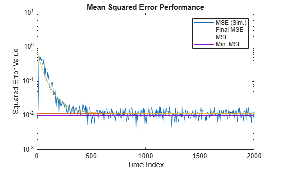
The predicted MSE follows the same trajectory as the simulated MSE. Both these trajectories converge with the steady-state (final) MSE.
Plot the Coefficient Trajectories
meanWsim is the mean value of the simulated coefficients given by msesim. meanW is the mean value of the predicted coefficients given by msepred.
Compare the simulated and predicted mean values of LMS filter coefficients 12,13,14, and 15.
plot(nn,meanWsim(:,12),'b',nn,meanW(:,12),'r',nn,...
meanWsim(:,13:15),'b',nn,meanW(:,13:15),'r')
PlotTitle ={'Average Coefficient Trajectories for';...
            'W(12), W(13), W(14), and W(15)'}
PlotTitle = 2×1 cell
    {'Average Coefficient Trajectories for'}
    {'W(12), W(13), W(14), and W(15)'      }
title(PlotTitle)
legend('Simulation','Theory')
xlabel('Time Index')
ylabel('Coefficient Value')
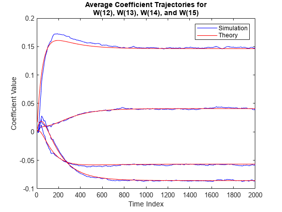
In steady state, both the trajectories converge.
Sum of Squared Coefficient Errors
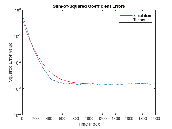
Compare the sum of the squared coefficient errors given by msepred and msesim. These values are given by the trace of the coefficient covariance matrix.
semilogy(nn,traceKsim,nn,traceK,'r')
title('Sum-of-Squared Coefficient Errors')
axis([0 size(x,1) 0.0001 1])
legend('Simulation','Theory')
xlabel('Time Index')
ylabel('Squared Error Value')
The maxstep function computes the maximum step size of the adaptive filter. This step size keeps the filter stable at the maximum possible speed of convergence. Create the primary input signal, x, by passing a signed random signal to an IIR filter. Signal x contains 50 frames of 2000 samples each frame. Create an LMS filter with 32 taps and a step size of 0.1.
x = zeros(2000,50);
IIRFilter = dsp.IIRFilter('Numerator',sqrt(0.75),...
    'Denominator',[1 -0.5]);
for k = 1:size(x,2)
  x(:,k) = IIRFilter(sign(randn(size(x,1),1)));
end
mu = 0.1;
LMSFilter = dsp.LMSFilter('Length',32,...
    'StepSize',mu);
Compute the maximum adaptation step size and the maximum step size in mean-squared sense using the maxstep function.
[mumax,mumaxmse] = maxstep(LMSFilter,x)
mumax =
0.0625
mumaxmse =
0.0536
System identification is the process of identifying the coefficients of an unknown system using an adaptive filter. The general overview of the process is shown in System Identification –– Using an Adaptive Filter to Identify an Unknown System. The main components involved are:
The adaptive filter algorithm. In this example, set the
Methodproperty ofdsp.LMSFilterto'LMS'to choose the LMS adaptive filter algorithm.An unknown system or process to adapt to. In this example, the filter designed by
fircbandis the unknown system.Appropriate input data to exercise the adaptation process. For the generic LMS model, these are the desired signal and the input signal .
The objective of the adaptive filter is to minimize the error signal between the output of the adaptive filter and the output of the unknown system (or the system to be identified) . Once the error signal is minimized, the adapted filter resembles the unknown system. The coefficients of both the filters match closely.
Unknown System
Create a dsp.FIRFilter object that represents the system to be identified. Use the fircband function to design the filter coefficients. The designed filter is a lowpass filter constrained to 0.2 ripple in the stopband.
filt = dsp.FIRFilter;
filt.Numerator = fircband(12,[0 0.4 0.5 1],[1 1 0 0],[1 0.2],...
{'w' 'c'});
Pass the signal x to the FIR filter. The desired signal d is the sum of the output of the unknown system (FIR filter) and an additive noise signal n.
x = 0.1*randn(250,1);
n = 0.01*randn(250,1);
d = filt(x) + n;
Adaptive Filter
With the unknown filter designed and the desired signal in place, create and apply the adaptive LMS filter object to identify the unknown filter.
Preparing the adaptive filter object requires starting values for estimates of the filter coefficients and the LMS step size (mu). You can start with some set of nonzero values as estimates for the filter coefficients. This example uses zeros for the 13 initial filter weights. Set the InitialConditions property of dsp.LMSFilter to the desired initial values of the filter weights. For the step size, 0.8 is a good compromise between being large enough to converge well within 250 iterations (250 input sample points) and small enough to create an accurate estimate of the unknown filter.
Create a dsp.LMSFilter object to represent an adaptive filter that uses the LMS adaptive algorithm. Set the length of the adaptive filter to 13 taps and the step size to 0.8.
mu = 0.8;
lms = dsp.LMSFilter(13,'StepSize',mu)
lms =
dsp.LMSFilter with properties:
Method: 'LMS'
Length: 13
StepSizeSource: 'Property'
StepSize: 0.8000
LeakageFactor: 1
InitialConditions: 0
AdaptInputPort: false
WeightsResetInputPort: false
WeightsOutput: 'Last'
Show all properties
Pass the primary input signal x and the desired signal d to the LMS filter. Run the adaptive filter to determine the unknown system. The output y of the adaptive filter is the signal converged to the desired signal d thereby minimizing the error e between the two signals.
Plot the results. The output signal does not match the desired signal as expected, making the error between the two nontrivial.
[y,e,w] = lms(x,d);
plot(1:250, [d,y,e])
title('System Identification of an FIR filter')
legend('Desired','Output','Error')
xlabel('Time index')
ylabel('Signal value')

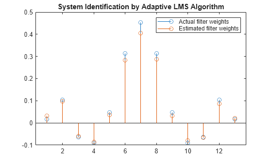
Compare the Weights
The weights vector w represents the coefficients of the LMS filter that is adapted to resemble the unknown system (FIR filter). To confirm the convergence, compare the numerator of the FIR filter and the estimated weights of the adaptive filter.
The estimated filter weights do not closely match the actual filter weights, confirming the results seen in the previous signal plot.
stem([(filt.Numerator).' w])
title('System Identification by Adaptive LMS Algorithm')
legend('Actual filter weights','Estimated filter weights',...
       'Location','NorthEast')
Changing the Step Size
As an experiment, change the step size to 0.2. Repeating the example with mu = 0.2 results in the following stem plot. The filters do not converge, and the estimated weights are not good approximations of the actual weights.
mu = 0.2;
lms = dsp.LMSFilter(13,'StepSize',mu);
[~,~,w] = lms(x,d);
stem([(filt.Numerator).' w])
title('System Identification by Adaptive LMS Algorithm')
legend('Actual filter weights','Estimated filter weights',...
       'Location','NorthEast')

Increase the Number of Data Samples
Increase the frame size of the desired signal. Even though this increases the computation involved, the LMS algorithm now has more data that can be used for adaptation. With 1000 samples of signal data and a step size of 0.2, the coefficients are aligned closer than before, indicating an improved convergence.
release(filt);
x = 0.1*randn(1000,1);
n = 0.01*randn(1000,1);
d = filt(x) + n;
[y,e,w] = lms(x,d);
stem([(filt.Numerator).' w])
title('System Identification by Adaptive LMS Algorithm')
legend('Actual filter weights','Estimated filter weights',...
       'Location','NorthEast')

Increase the number of data samples further by inputting the data through iterations. Run the algorithm on 4000 samples of data, passed to the LMS algorithm in batches of 1000 samples over 4 iterations.
Compare the filter weights. The weights of the LMS filter match the weights of the FIR filter very closely, indicating a good convergence.
release(filt);
n = 0.01*randn(1000,1);
for index = 1:4
  x = 0.1*randn(1000,1);
  d = filt(x) + n;
  [y,e,w] = lms(x,d);
end
stem([(filt.Numerator).' w])
title('System Identification by Adaptive LMS Algorithm')
legend('Actual filter weights','Estimated filter weights',...
       'Location','NorthEast')

The output signal matches the desired signal very closely, making the error between the two close to zero.
plot(1:1000, [d,y,e])
title('System Identification of an FIR filter')
legend('Desired','Output','Error')
xlabel('Time index')
ylabel('Signal value')

To improve the convergence performance of the LMS algorithm, the normalized variant (NLMS) uses an adaptive step size based on the signal power. As the input signal power changes, the algorithm calculates the input power and adjusts the step size to maintain an appropriate value. The step size changes with time, and as a result, the normalized algorithm converges faster with fewer samples in many cases. For input signals that change slowly over time, the normalized LMS algorithm can be a more efficient LMS approach.
For an example using the LMS approach, see System Identification of FIR Filter Using LMS Algorithm.
Unknown System
Create a dsp.FIRFilter object that represents the system to be identified. Use the fircband function to design the filter coefficients. The designed filter is a lowpass filter constrained to 0.2 ripple in the stopband.
filt = dsp.FIRFilter;
filt.Numerator = fircband(12,[0 0.4 0.5 1],[1 1 0 0],[1 0.2],...
{'w' 'c'});
Pass the signal x to the FIR filter. The desired signal d is the sum of the output of the unknown system (FIR filter) and an additive noise signal n.
x = 0.1*randn(1000,1);
n = 0.001*randn(1000,1);
d = filt(x) + n;
Adaptive Filter
To use the normalized LMS algorithm variation, set the Method property on the dsp.LMSFilter to 'Normalized LMS'. Set the length of the adaptive filter to 13 taps and the step size to 0.2.
mu = 0.2;
lms = dsp.LMSFilter(13,'StepSize',mu,'Method',...
   'Normalized LMS');
Pass the primary input signal x and the desired signal d to the LMS filter.
[y,e,w] = lms(x,d);
The output y of the adaptive filter is the signal converged to the desired signal d thereby minimizing the error e between the two signals.
plot(1:1000, [d,y,e])
title('System Identification by Normalized LMS Algorithm')
legend('Desired','Output','Error')
xlabel('Time index')
ylabel('Signal value')
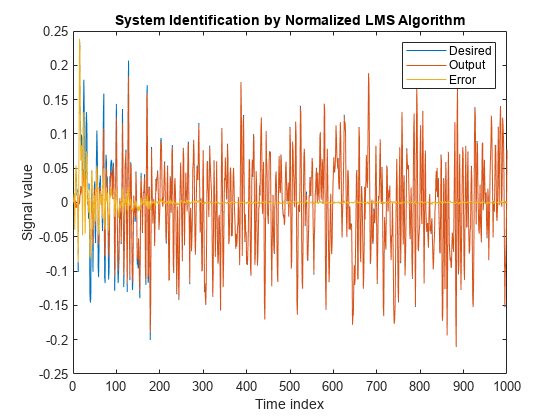
Compare the Adapted Filter to the Unknown System
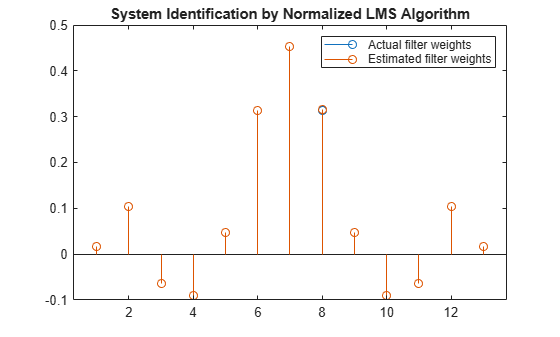
The weights vector w represents the coefficients of the LMS filter that is adapted to resemble the unknown system (FIR filter). To confirm the convergence, compare the numerator of the FIR filter and the estimated weights of the adaptive filter.
stem([(filt.Numerator).' w])
title('System Identification by Normalized LMS Algorithm')
legend('Actual filter weights','Estimated filter weights',...
       'Location','NorthEast')
An adaptive filter adapts its filter coefficients to match the coefficients of an unknown system. The objective is to minimize the error signal between the output of the unknown system and the output of the adaptive filter. When these two outputs converge and match closely for the same input, the coefficients are said to match closely. The adaptive filter at this state resembles the unknown system. This example compares the rate at which this convergence happens for the normalized LMS (NLMS) algorithm and the LMS algorithm with no normalization.
Unknown System
Create a dsp.FIRFilter that represents the unknown system. Pass the signal x as an input to the unknown system. The desired signal d is the sum of the output of the unknown system (FIR filter) and an additive noise signal n.
filt = dsp.FIRFilter;
filt.Numerator = fircband(12,[0 0.4 0.5 1],[1 1 0 0],[1 0.2],...
{'w' 'c'});
x = 0.1*randn(1000,1);
n = 0.001*randn(1000,1);
d = filt(x) + n;
Adaptive Filter
Create two dsp.LMSFilter objects, with one set to the LMS algorithm, and the other set to the normalized LMS algorithm. Choose an adaptation step size of 0.2 and set the length of the adaptive filter to 13 taps.
mu = 0.2;
lms_nonnormalized = dsp.LMSFilter(13,'StepSize',mu,...
    'Method','LMS');
lms_normalized = dsp.LMSFilter(13,'StepSize',mu,...
    'Method','Normalized LMS');
Pass the primary input signal x and the desired signal d to both the variations of the LMS algorithm. The variables e1 and e2 represent the error between the desired signal and the output of the normalized and nonnormalized filters, respectively.
[~,e1,~] = lms_normalized(x,d);
[~,e2,~] = lms_nonnormalized(x,d);
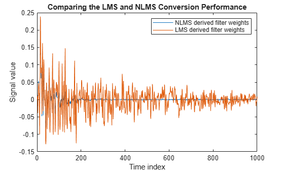
Plot the error signals for both variations. The error signal for the NLMS variant converges to zero much faster than the error signal for the LMS variant. The normalized version adapts in far fewer iterations to a result almost as good as the nonnormalized version.
plot([e1,e2]);
title('Comparing the LMS and NLMS Conversion Performance');
legend('NLMS derived filter weights', ...
       'LMS derived filter weights','Location', 'NorthEast');
xlabel('Time index')
ylabel('Signal value')
Cancel additive noise, n, added to an unknown system using an LMS adaptive filter. The LMS filter adapts its coefficients until its transfer function matches the transfer function of the unknown system as closely as possible. The difference between the output of the adaptive filter and the output of the unknown system represents the error signal, e. Minimizing this error signal is the objective of the adaptive filter.
The unknown system and the LMS filter process the same input signal, x, and produce outputs d and y, respectively. If the coefficients of the adaptive filter match the coefficients of the unknown system, the error, e, in effect represents the additive noise.
Create a dsp.FIRFilter System object to represent the unknown system. Create a dsp.LMSFilter object and set the length to 11 taps and the step size to 0.05. Create a sine wave to represent the noise added to the unknown system. View the signals in a time scope.
FrameSize = 100;
NIter = 10;
lmsfilt2 = dsp.LMSFilter('Length',11,'Method','Normalized LMS', ...
    'StepSize',0.05);
firfilt2 = dsp.FIRFilter('Numerator', fir1(10,[.5, .75]));
sinewave = dsp.SineWave('Frequency',0.01, ...
    'SampleRate',1,'SamplesPerFrame',FrameSize);
scope = timescope('TimeUnits','Seconds',...
    'YLimits',[-3 3],'BufferLength',2*FrameSize*NIter, ...
    'ShowLegend',true,'ChannelNames', ...
    {'Noisy signal', 'Error signal'});
Create a random input signal, x and pass the signal to the FIR filter. Add a sine wave to the output of the FIR filter to generate the noisy signal, d. The signal, d is the output of the unknown system. Pass the noisy signal and the primary input signal to the LMS filter. View the noisy signal and the error signal in the time scope.
for k = 1:NIter
    x = randn(FrameSize,1);
    d = firfilt2(x) + sinewave();
    [y,e,w] = lmsfilt2(x,d);
    scope([d,e])
end
release(scope)
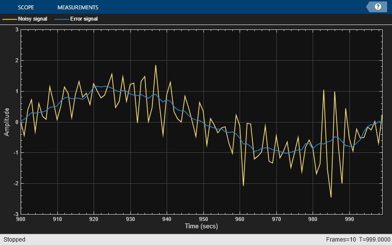
The error signal, e, is the sinusoidal noise added to the unknown system. Minimizing the error signal minimizes the noise added to the system.
When the amount of computation required to derive an adaptive filter drives your development process, the sign-data variant of the LMS (SDLMS) algorithm might be a very good choice, as demonstrated in this example.
In the standard and normalized variations of the LMS adaptive filter, coefficients for the adapting filter arise from the mean square error between the desired signal and the output signal from the unknown system. The sign-data algorithm changes the mean square error calculation by using the sign of the input data to change the filter coefficients.
When the error is positive, the new coefficients are the previous coefficients plus the error multiplied by the step size µ. If the error is negative, the new coefficients are again the previous coefficients minus the error multiplied by µ — note the sign change.
When the input is zero, the new coefficients are the same as the previous set.
In vector form, the sign-data LMS algorithm is:
where
with vector containing the weights applied to the filter coefficients and vector containing the input data. The vector is the error between the desired signal and the filtered signal. The objective of the SDLMS algorithm is to minimize this error. Step size is represented by .
With a smaller , the correction to the filter weights gets smaller for each sample, and the SDLMS error falls more slowly. A larger changes the weights more for each step, so the error falls more rapidly, but the resulting error does not approach the ideal solution as closely. To ensure a good convergence rate and stability, select within the following practical bounds.
where is the number of samples in the signal. Also, define as a power of two for efficient computing.
Note: How you set the initial conditions of the sign-data algorithm profoundly influences the effectiveness of the adaptation process. Because the algorithm essentially quantizes the input signal, the algorithm can become unstable easily.
A series of large input values, coupled with the quantization process might result in the error growing beyond all bounds. Restrain the tendency of the sign-data algorithm to get out of control by choosing a small step size and setting the initial conditions for the algorithm to nonzero positive and negative values.
In this noise cancellation example, set the Method property of dsp.LMSFilter to 'Sign-Data LMS'. This example requires two input data sets:
Data containing a signal corrupted by noise. In the block diagram under Noise or Interference Cancellation –– Using an Adaptive Filter to Remove Noise from an Unknown System, this is the desired signal . The noise cancellation process removes the noise from the signal.
Data containing random noise. In the block diagram under Noise or Interference Cancellation –– Using an Adaptive Filter to Remove Noise from an Unknown System, this is . The signal is correlated with the noise that corrupts the signal data. Without the correlation between the noise data, the adapting algorithm cannot remove the noise from the signal.
For the signal, use a sine wave. Note that signal is a column vector of 1000 elements.
signal = sin(2*pi*0.055*(0:1000-1)');
Now, add correlated white noise to signal. To ensure that the noise is correlated, pass the noise through a lowpass FIR filter and then add the filtered noise to the signal.
noise = randn(1000,1);
filt = dsp.FIRFilter;
filt.Numerator = fir1(11,0.4);
fnoise = filt(noise);
d = signal + fnoise;
fnoise is the correlated noise and d is now the desired input to the sign-data algorithm.
To prepare the dsp.LMSFilter object for processing, set the initial conditions of the filter weights and mu (StepSize). As noted earlier in this section, the values you set for coeffs and mu determine whether the adaptive filter can remove the noise from the signal path.
In System Identification of FIR Filter Using LMS Algorithm, you constructed a default filter that sets the filter coefficients to zeros. In most cases that approach does not work for the sign-data algorithm. The closer you set your initial filter coefficients to the expected values, the more likely it is that the algorithm remains well behaved and converges to a filter solution that removes the noise effectively.
For this example, start with the coefficients used in the noise filter (filt.Numerator), and modify them slightly so the algorithm has to adapt.
coeffs = (filt.Numerator).'-0.01; % Set the filter initial conditions.
mu = 0.05; % Set the step size for algorithm updating.
With the required input arguments for dsp.LMSFilter prepared, construct the LMS filter object, run the adaptation, and view the results.
lms = dsp.LMSFilter(12,'Method','Sign-Data LMS',...
   'StepSize',mu,'InitialConditions',coeffs);
[~,e] = lms(noise,d);
L = 200;
plot(0:L-1,signal(1:L),0:L-1,e(1:L));
title('Noise Cancellation by the Sign-Data Algorithm');
legend('Actual signal','Result of noise cancellation',...
       'Location','NorthEast');
xlabel('Time index')
ylabel('Signal values')

When dsp.LMSFilter runs, it uses far fewer multiplication operations than either of the standard LMS algorithms. Also, performing the sign-data adaptation requires only multiplication by bit shifting when the step size is a power of two.
Although the performance of the sign-data algorithm as shown in this plot is quite good, the sign-data algorithm is much less stable than the standard LMS variations. In this noise cancellation example, the processed signal is a very good match to the input signal, but the algorithm could very easily grow without bound rather than achieve good performance.
Changing the weight initial conditions (InitialConditions) and mu (StepSize), or even the lowpass filter you used to create the correlated noise, can cause noise cancellation to fail.
In the standard and normalized variations of the LMS adaptive filter, the coefficients for the adapting filter arise from calculating the mean square error between the desired signal and the output signal from the unknown system, and applying the result to the current filter coefficients. The sign-error LMS (SELMS) algorithm replaces the mean square error calculation by using the sign of the error to modify the filter coefficients.
When the error is positive, the new coefficients are the previous coefficients plus the error multiplied by the step size . If the error is negative, the new coefficients are the previous coefficients minus the error multiplied by — note the sign change. When the input is zero, the new coefficients are the same as the previous set.
In vector form, the sign-error LMS algorithm is:
,
where
with vector containing the weights applied to the filter coefficients and vector containing the input data. The vector is the error between the desired signal and the filtered signal. The objective of the SELMS algorithm is to minimize this error.
With a smaller , the correction to the filter weights gets smaller for each sample and the SELMS error falls more slowly. A larger changes the weights more for each step so the error falls more rapidly, but the resulting error does not approach the ideal solution as closely. To ensure a good convergence rate and stability, select within the following practical bounds.
where is the number of samples in the signal. Also, define as a power of two for efficient computation.
Note: How you set the initial conditions of the sign-error algorithm profoundly influences the effectiveness of the adaptation process. Because the algorithm essentially quantizes the error signal, the algorithm can become unstable easily.
A series of large error values, coupled with the quantization process might result in the error growing beyond all bounds. Restrain the tendency of the sign-error algorithm to become unstable by choosing a small step size and setting the initial conditions for the algorithm to nonzero positive and negative values.
In this noise cancellation example, set the Method property of dsp.LMSFilter to 'Sign-Error LMS'. This example requires two input data sets:
Data containing a signal corrupted by noise. In the block diagram under Noise or Interference Cancellation –– Using an Adaptive Filter to Remove Noise from an Unknown System, this is the desired signal . The noise cancellation process removes the noise from the signal.
Data containing random noise. In the block diagram under Noise or Interference Cancellation –– Using an Adaptive Filter to Remove Noise from an Unknown System, this is . The signal is correlated with the noise that corrupts the signal data. Without the correlation between the noise data, the adapting algorithm cannot remove the noise from the signal.
For the signal, use a sine wave. Note that signal is a column vector of 1000 elements.
signal = sin(2*pi*0.055*(0:1000-1)');
Now, add correlated white noise to signal. To ensure that the noise is correlated, pass the noise through a lowpass FIR filter and then add the filtered noise to the signal.
noise = randn(1000,1);
filt = dsp.FIRFilter;
filt.Numerator = fir1(11,0.4);
fnoise = filt(noise);
d = signal + fnoise;
fnoise is the correlated noise and d is now the desired input to the sign-error algorithm.
To prepare the dsp.LMSFilter object for processing, set the initial conditions of the filter weights (InitialConditions) and mu (StepSize). As noted earlier in this section, the values you set for coeffs and mu determine whether the adaptive filter can remove the noise from the signal path.
In System Identification of FIR Filter Using LMS Algorithm, you constructed a default filter that sets the filter coefficients to zeros. In most cases that approach does not work for the sign-error algorithm. The closer you set your initial filter coefficients to the expected values, the more likely it is that the algorithm remains well behaved and converges to a filter solution that removes the noise effectively.
For this example, start with the coefficients used in the noise filter (filt.Numerator) and modify them slightly so the algorithm has to adapt.
coeffs = (filt.Numerator).'-0.01; % Set the filter initial conditions.
mu = 0.05; % Set the step size for algorithm updating.
With the required input arguments for dsp.LMSFilter prepared, run the adaptation and view the results.
lms = dsp.LMSFilter(12,'Method','Sign-Error LMS',...
   'StepSize',mu,'InitialConditions',coeffs);
[~,e] = lms(noise,d);
L = 200;
plot(0:199,signal(1:200),0:199,e(1:200));
title('Noise cancellation performance by the sign-error LMS algorithm');
legend('Actual signal','Error after noise reduction',...
       'Location','NorthEast')
xlabel('Time index')
ylabel('Signal value')

When the sign-error LMS algorithm runs, it uses far fewer multiplication operations than either of the standard LMS algorithms. Also, performing the sign-error adaptation requires only bit shifting multiples when the step size is a power of two.
Although the performance of the sign-error algorithm as shown in this plot is quite good, the sign-error algorithm is much less stable than the standard LMS variations. In this noise cancellation example, the adapted signal is a very good match to the input signal, but the algorithm could very easily become unstable rather than achieve good performance.
Changing the weight initial conditions (InitialConditions) and mu (StepSize), or even the lowpass filter you used to create the correlated noise, can cause noise cancellation to fail and the algorithm to become useless.
The sign-sign LMS algorithm (SSLMS) replaces the mean square error calculation by using the sign of the input data to change the filter coefficients. When the error is positive, the new coefficients are the previous coefficients plus the error multiplied by the step size . If the error is negative, the new coefficients are the previous coefficients minus the error multiplied by — note the sign change. When the input is zero, the new coefficients are the same as the previous set.
In essence, the algorithm quantizes both the error and the input by applying the sign operator to them.
In vector form, the sign-sign LMS algorithm is:
where
Vector contains the weights applied to the filter coefficients and vector contains the input data. The vector is the error between the desired signal and the filtered signal. The objective of the SSLMS algorithm is to minimize this error.
With a smaller , the correction to the filter weights gets smaller for each sample and the SSLMS error falls more slowly. A larger changes the weights more for each step, so the error falls more rapidly, but the resulting error does not approach the ideal solution as closely. To ensure a good convergence rate and stability, select within the following practical bounds.
where is the number of samples in the signal. Also, define as a power of two for efficient computation
Note:
How you set the initial conditions of the sign-sign algorithm profoundly influences the effectiveness of the adaptation process. Because the algorithm essentially quantizes the input signal and the error signal, the algorithm can become unstable easily.
A series of large error values, coupled with the quantization process might result in the error growing beyond all bounds. Restrain the tendency of the sign-sign algorithm to become unstable by choosing a small step size and setting the initial conditions for the algorithm to nonzero positive and negative values.
In this noise cancellation example, set the Method property of dsp.LMSFilter to 'Sign-Sign LMS'. This example requires two input data sets:
Data containing a signal corrupted by noise. In the block diagram under Noise or Interference Cancellation –– Using an Adaptive Filter to Remove Noise from an Unknown System, this is the desired signal . The noise cancellation process removes the noise from the signal.
Data containing random noise. In the block diagram under Noise or Interference Cancellation –– Using an Adaptive Filter to Remove Noise from an Unknown System, this is . The signal is correlated with the noise that corrupts the signal data. Without the correlation between the noise data, the adapting algorithm cannot remove the noise from the signal.
For the signal, use a sine wave. Note that signal is a column vector of 1000 elements.
signal = sin(2*pi*0.055*(0:1000-1)');
Now, add correlated white noise to signal. To ensure that the noise is correlated, pass the noise through a lowpass FIR filter, then add the filtered noise to the signal.
noise = randn(1000,1);
filt = dsp.FIRFilter;
filt.Numerator = fir1(11,0.4);
fnoise = filt(noise);
d = signal + fnoise;
fnoise is the correlated noise and d is now the desired input to the sign-sign algorithm.
To prepare the dsp.LMSFilter object for processing, set the initial conditions of the filter weights (InitialConditions) and mu (StepSize). As noted earlier in this section, the values you set for coeffs and mu determine whether the adaptive filter can remove the noise from the signal path. In System Identification of FIR Filter Using LMS Algorithm, you constructed a default filter that sets the filter coefficients to zeros. Usually that approach does not work for the sign-sign algorithm.
The closer you set your initial filter coefficients to the expected values, the more likely it is that the algorithm remains well behaved and converges to a filter solution that removes the noise effectively. For this example, you start with the coefficients used in the noise filter (filt.Numerator), and modify them slightly so the algorithm has to adapt.
coeffs = (filt.Numerator).' -0.01; % Set the filter initial conditions.
mu = 0.05;
With the required input arguments for dsp.LMSFilter prepared, run the adaptation and view the results.
lms = dsp.LMSFilter(12,'Method','Sign-Sign LMS',...
   'StepSize',mu,'InitialConditions',coeffs);
[~,e] = lms(noise,d);
L = 200;
plot(0:199,signal(1:200),0:199,e(1:200));
title('Noise cancellation performance by the sign-sign LMS algorithm');
legend('Actual signal','Error after noise reduction',...
       'Location','NorthEast')
xlabel('Time index')
ylabel('Signal value')

When dsp.LMSFilter runs, it uses far fewer multiplication operations than either of the standard LMS algorithms. Also, performing the sign-sign adaptation requires only bit shifting multiples when the step size is a power of two.
Although the performance of the sign-sign algorithm as shown in this plot is quite good, the sign-sign algorithm is much less stable than the standard LMS variations. In this noise cancellation example, the adapted signal is a very good match to the input signal, but the algorithm could very easily become unstable rather than achieve good performance.
Changing the weight initial conditions (InitialConditions) and mu (StepSize), or even the lowpass filter you used to create the correlated noise, can cause noise cancellation to fail and the algorithm to become useless.
Note: This example runs only in R2017a or later. If you are using a release earlier than R2017a, the object does not output a full sample-by-sample history of filter weights.
Initialize the dsp.LMSFilter System object and set the WeightsOutput property to 'All'. This setting enables the LMS filter to output a matrix of weights with dimensions [FrameLength Length], corresponding to the full sample-by-sample history of weights for all FrameLength samples of input values.
FrameSize = 15000;
lmsfilt3 = dsp.LMSFilter('Length',63,'Method','LMS', ...
    'StepSize',0.001,'LeakageFactor',0.99999, ...
    'WeightsOutput','All'); % full Weights history

w_actual = fir1(64,[0.5 0.75]);
firfilt3 = dsp.FIRFilter('Numerator',w_actual);
sinewave = dsp.SineWave('Frequency',0.01, ...
    'SampleRate',1,'SamplesPerFrame',FrameSize);

scope = timescope('TimeUnits','Seconds', ...
    'YLimits',[-0.25 0.75],'BufferLength',2*FrameSize, ...
    'ShowLegend',true,'ChannelNames', ...
    {'Coeff 33 Estimate','Coeff 34 Estimate','Coeff 35 Estimate', ...
    'Coeff 33 Actual','Coeff 34 Actual','Coeff 35 Actual'});
Run one frame and output the full adaptive weights history, w.
x = randn(FrameSize,1);       % Input signal
d = firfilt3(x) + sinewave(); % Noise + Signal
[~,~,w] = lmsfilt3(x,d);
Each row in w is a set of weights estimated for the respective input sample. Each column in w gives the complete history of a specific weight. Plot the actual weight and the entire history of the 33rd, 34th, and 35th weight. In the plot, you can see that the estimated weight output eventually converges with the actual weight as the adaptive filter receives input samples and continues to adapt.
idxBeg = 33;
idxEnd = 35;
scope([w(:,idxBeg:idxEnd), repmat(w_actual(idxBeg:idxEnd),FrameSize,1)])

More About
The following diagrams show the data types used within the
dsp.LMSFilter object for fixed-point signals. The table summarizes the
definitions of the variables used in the diagrams:
| Variable | Definition |
|---|---|
u | Input vector |
W | Vector of filter weights |
µ | Step size |
e | Error |
Q | Quotient, |
Product u'u | Product data type in Energy calculation diagram |
Accumulator u'u | Accumulator data type in Energy calculation diagram |
Product W'u | Product data type in Convolution diagram |
Accumulator W'u | Accumulator data type in Convolution diagram |
Product | Product data type in Product of step size and error diagram |
Product | Product and accumulator data type in Weight update diagram. 1 |
1The accumulator data type for this quantity is automatically set to be the same as the product data type. The minimum, maximum, and overflow information for this accumulator is logged as part of the product information. Autoscaling treats this product and accumulator as one data type.


You can set the data type of the properties, weights, products, quotient, and accumulators in the System object properties. Fixed-point inputs, outputs, and System object properties must have the following characteristics:
The input signal and the desired signal must have the same word length, but their fraction lengths can differ.
The step size and leakage factor must have the same word length, but their fraction lengths can differ.
The output signal and the error signal have the same word length and the same fraction length as the desired signal.
The quotient and the product output of the u'u, W'u, , and operations must have the same word length, but their fraction lengths can differ.
The accumulator data type of the u'u and W'u operations must have the same word length, but their fraction lengths can differ.
The output of the multiplier is in the product output data type if at least one of the inputs to the multiplier is real. If both of the inputs to the multiplier are complex, the result of the multiplication is in the accumulator data type. For details on the complex multiplication performed, see Multiplication Data Types.
Algorithms
The LMS filter algorithm is defined by the following equations.
The various LMS adaptive filter algorithms available in this System object are defined as:
LMS –– Solves the Wiener-Hopf equation and finds the filter coefficients for an adaptive filter.
Normalized LMS –– Normalized variation of the LMS algorithm.
In Normalized LMS, to overcome potential numerical instability in the update of the weights, a small positive constant, ε, has been added in the denominator. For double-precision floating-point input, ε is the output of the
epsfunction. For single-precision floating-point input, ε is the output ofeps("single"). For fixed-point input, ε is 0.Sign-Data LMS –– Correction to the filter weights at each iteration depends on the sign of the input u(n).
where u(n) is real.
Sign-Error LMS –– Correction applied to the current filter weights for each successive iteration depends on the sign of the error, e(n).
Sign-Sign LMS –– Correction applied to the current filter weights for each successive iteration depends on both the sign of u(n) and the sign of e(n).
where u(n) is real.
The variables are as follows:
| Variable | Description |
|---|---|
|
n |
The current time index |
|
u(n) |
The vector of buffered input samples at step n |
|
u*(n) |
The complex conjugate of the vector of buffered input samples at step n |
|
w(n) |
The vector of filter weight estimates at step n |
|
y(n) |
The filtered output at step n |
|
e(n) |
The estimation error at step n |
|
d(n) |
The desired response at step n |
|
µ |
The adaptation step size |
α | The leakage factor (0 < α ≤ 1) |
ε | A constant that corrects any potential numerical instability that occurs during the update of weights. |
References
[1] Hayes, M.H. Statistical Digital Signal Processing and Modeling. New York: John Wiley & Sons, 1996.
Extended Capabilities
Version History
Introduced in R2012aSee Also
Functions
Objects
dsp.BlockLMSFilter|dsp.FIRFilter|dsp.FilteredXLMSFilter|dsp.FrequencyDomainAdaptiveFilter|dsp.AdaptiveLatticeFilter|dsp.AffineProjectionFilter|dsp.FastTransversalFilter|dsp.RLSFilter