Main Content

dsp.AffineProjectionFilter

Compute output, error and coefficients using affine projection (AP) Algorithm

Description

The dsp.AffineProjectionFilter System object™ filters each channel of the input using AP filter implementations.

To filter each channel of the input:

  1. Create the dsp.AffineProjectionFilter object and set its properties.

  2. Call the object with arguments, as if it were a function.

To learn more about how System objects work, see What Are System Objects?

Creation

Description

apf = dsp.AffineProjectionFilter returns an adaptive FIR filter System object, apf. This System object computes the filtered output and the filter error for a given input and desired signal using the affine projection (AP) algorithm.

example

apf = dsp.AffineProjectionFilter(len) returns an affine projection filter object with the Length property set to len.

example

apf = dsp.AffineProjectionFilter(Name,Value) returns an affine projection filter object with each specified property set to the specified value. Enclose each property name in single quotes. Unspecified properties have default values.

Properties

expand all

Unless otherwise indicated, properties are nontunable, which means you cannot change their values after calling the object. Objects lock when you call them, and the release function unlocks them.

If a property is tunable, you can change its value at any time.

For more information on changing property values, see System Design in MATLAB Using System Objects.

Specify the method used to calculate filter coefficients as Direct Matrix Inversion, Recursive Matrix Update, Block Direct Matrix Inversion. This property is nontunable.

Specify the length of the FIR filter coefficients vector as a scalar positive integer value. This property is nontunable.

Data Types: single | double | int8 | int16 | int32 | int64 | uint8 | uint16 | uint32 | uint64

Specify the projection order of the affine projection algorithm as a scalar positive integer value greater than or equal to 2. This property defines the size of the input signal covariance matrix. This property is nontunable.

Data Types: double

Specify the affine projection step size factor as a scalar nonnegative numeric value between 0 and 1, both inclusive. Setting the step size equal to one provides the fastest convergence during adaptation.

Tunable: Yes

Data Types: single | double | int8 | int16 | int32 | int64 | uint8 | uint16 | uint32 | uint64 | logical

Specify the initial values of the FIR adaptive filter coefficients as a scalar or a vector of length equal to the Length property value.

Tunable: Yes

Data Types: single | double | int8 | int16 | int32 | int64 | uint8 | uint16 | uint32 | uint64

Specify the initial values for the offset input covariance matrix. This property must be either a scalar positive numeric value or a positive-definite square matrix with each dimension equal to the ProjectionOrder property value. If it is a scalar value, the OffsetCovariance property is initialized to a diagonal matrix with the diagonal elements equal to that scalar value. If it is a square matrix, the OffsetCovariance property is initialized to the value of that square matrix.

Tunable: Yes

Dependencies

This property is applicable only if the Method property is set to Direct Matrix Inversion or Block Direct Matrix Inversion.

Data Types: single | double | int8 | int16 | int32 | int64 | uint8 | uint16 | uint32 | uint64

Specify the initial values for the offset input covariance matrix inverse. This property must be either a scalar positive numeric value or a positive-definite square matrix with each dimension equal to the ProjectionOrder property value. If it is a scalar value, the InverseOffsetCovariance property is initialized to a diagonal matrix with each diagonal element equal to that scalar value. If it is a square matrix, the InverseOffsetCovariance property is initialized to the values of that square matrix.

Tunable: Yes

Dependencies

This property is applicable only if the Method property is set to Recursive Matrix Update.

Data Types: single | double | int8 | int16 | int32 | int64 | uint8 | uint16 | uint32 | uint64

Specify the initial values of the correlation coefficients of the FIR filter as a scalar or a vector of length equal to ProjectionOrder1.

Tunable: Yes

Dependencies

This property is applicable only if the Method property is set to Recursive Matrix Update.

Data Types: single | double | int8 | int16 | int32 | int64 | uint8 | uint16 | uint32 | uint64

Specify whether the filter coefficient values should be locked. When you set this property to true, the filter coefficients are not updated and their values remain the same. The default value is false (filter coefficients are continuously updated).

Tunable: Yes

Usage

Description

example

[y,err] = apf(x,d) filters the input x, using d as the desired signal, and returns the filtered output in y and the filter error in err. The System object estimates the filter weights needed to minimize the error between the output signal and the desired signal. You can access these coefficients by accessing the Coefficients property of the object. This can be done only after calling the object. For example, to access the optimized coefficients of the apf filter, call apf.Coefficients after you pass the input and desired signal to the object.

Input Arguments

expand all

The signal to be filtered by the affine projection filter. The input, x, and the desired signal, d, must have the same size and data type.

The input can be a variable-size signal. You can change the number of elements in the column vector even when the object is locked. The System object locks when you call the object to run its algorithm.

Data Types: single | double
Complex Number Support: Yes

The affine projection filter adapts its coefficients to minimize the error, err, and converge the input signal x to the desired signal d as closely as possible.

The input, x, and the desired signal, d, must have the same size and data type.

The desired signal can be a variable-size signal. You can change the number of elements in the column vector even when the object is locked. The System object locks when you call the object.

Data Types: single | double
Complex Number Support: Yes

Output Arguments

expand all

Filtered output, returned as a scalar or a column vector. The object adapts its filter coefficients to converge the input signal x to match the desired signal d. The filter outputs the converged signal.

Data Types: single | double
Complex Number Support: Yes

Difference between the output signal y and the desired signal d, returned as a scalar or a column vector. The objective of the affine projection filter is to minimize this error. The object adapts its coefficients to converge towards optimal filter coefficients that produce an output signal that matches closely with the desired signal. To access the affine projection filter coefficients, call apf.Coefficients after you pass the input and desired signal to the object.

Data Types: single | double
Complex Number Support: Yes

Object Functions

To use an object function, specify the System object as the first input argument. For example, to release system resources of a System object named obj, use this syntax:

release(obj)

expand all

msesimEstimated mean squared error for adaptive filters
stepRun System object algorithm
releaseRelease resources and allow changes to System object property values and input characteristics
resetReset internal states of System object

Examples

collapse all

QPSK Adaptive Equalization Using a 32-Coefficient FIR Filter (1000 Iterations)

D = 16;                      % Number of samples of delay
b = exp(1i*pi/4)*[-0.7 1];    % Numerator coefficients of channel
a = [1 -0.7];                % Denominator coefficients of channel
ntr = 1000;                  % Number of iterations
s = sign(randn(1,ntr+D)) + 1i*sign(randn(1,ntr+D)); % Baseband signal
n = 0.1*(randn(1,ntr+D) + 1i*randn(1,ntr+D));       % Noise signal
r = filter(b,a,s)+n;         % Received signal
x = r(1+D:ntr+D);            % Input signal (received signal)
d = s(1:ntr);                % Desired signal (delayed QPSK signal)
mu = 0.1;                    % Step size
po = 4;                      % Projection order
offset = 0.05;               % Offset for covariance matrix
apf = dsp.AffineProjectionFilter('Length', 32, ...
    'StepSize', mu, 'ProjectionOrder', po, ...
    'InitialOffsetCovariance',offset);
[y,e] = apf(x,d);
subplot(2,2,1); plot(1:ntr,real([d;y;e]));
title('In-Phase Components');
legend('Desired','Output','Error');
xlabel('time index'); ylabel('signal value');
subplot(2,2,2); plot(1:ntr,imag([d;y;e]));
title('Quadrature Components');
legend('Desired','Output','Error');
xlabel('time index'); ylabel('signal value');
subplot(2,2,3); plot(x(ntr-100:ntr),'.'); axis([-3 3 -3 3]);
title('Received Signal Scatter Plot'); axis('square');
xlabel('Real[x]'); ylabel('Imag[x]'); grid on;
subplot(2,2,4); plot(y(ntr-100:ntr),'.'); axis([-3 3 -3 3]);
title('Equalized Signal Scatter Plot'); axis('square');
xlabel('Real[y]'); ylabel('Imag[y]'); grid on;

Figure contains 4 axes objects. Axes object 1 with title In-Phase Components, xlabel time index, ylabel signal value contains 3 objects of type line. These objects represent Desired, Output, Error. Axes object 2 with title Quadrature Components, xlabel time index, ylabel signal value contains 3 objects of type line. These objects represent Desired, Output, Error. axes object 3 with title Received Signal Scatter Plot, xlabel Real[x], ylabel Imag[x] contains a line object which displays its values using only markers. axes object 4 with title Equalized Signal Scatter Plot, xlabel Real[y], ylabel Imag[y] contains a line object which displays its values using only markers.

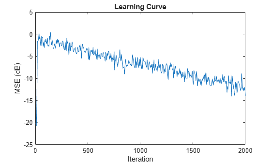
ha = fir1(31,0.5);
% FIR system to be identified 
fir = dsp.FIRFilter('Numerator',ha); 
iir = dsp.IIRFilter('Numerator',sqrt(0.75),...
        'Denominator',[1 -0.5]);
x = iir(sign(randn(2000,25))); 
% Observation noise signal 
n = 0.1*randn(size(x));         
% Desired signal 
d = fir(x)+n;  
% Filter length 
l = 32;  
% Affine Projection filter Step size. 
mu = 0.008;
% Decimation factor for analysis
% and simulation results 
m  = 5;                             
                                    
apf = dsp.AffineProjectionFilter(l,'StepSize',mu); 
[simmse,meanWsim,Wsim,traceKsim] = msesim(apf,x,d,m);
plot(m*(1:length(simmse)),10*log10(simmse));
xlabel('Iteration'); ylabel('MSE (dB)');
% Plot the learning curve for affine projection filter 
% used in system identification
title('Learning curve')

Figure contains an axes object. The axes object with title Learning curve, xlabel Iteration, ylabel MSE (dB) contains an object of type line.

Algorithms

The affine projection algorithm (APA) is an adaptive scheme that estimates an unknown system based on multiple input vectors [1]. It is designed to improve the performance of other adaptive algorithms, mainly those that are LMS based. The affine projection algorithm reuses old data resulting in fast convergence when the input signal is highly correlated, leading to a family of algorithms that can make trade-offs between computation complexity with convergence speed [2].

The following equations describe the conceptual algorithm used in designing AP filters:

Uap(n)=(u(n)u(nL)u(nN)u(nLN))=(u(n)u(n1)u(nL))yap(n)=UTap(n)w(n)=(y(n)···y(nL))dap(n)=(d(n)···d(nL))eap(n)=dap(n)yap(n)=(e(n)···e(nL))w(n)=w(n1)+μUap(n)(UapH(n)Uap(n)+C)1eap

where C is either εI if the initial offset covariance is a scalar ε, or R if the initial offset covariance is a matrix R. The variables are as follows:

VariableDescription
nThe current time index
u(n)The input sample at step n
Uap(n)The matrix of the last L+1 input signal vectors
w(n)The adaptive filter coefficients vector
y(n)The adaptive filter output
d(n)The desired signal
e(n)The error at step n
LThe projection order
NThe filter order (i.e., filter length = N+1)
μThe step size

References

[1] K. Ozeki, T. Umeda, “An adaptive Filtering Algorithm Using an Orthogonal Projection to an Affine Subspace and its Properties”, Electron. Commun. Jpn. 67-A(5), May 1984, pp. 19–27.

[2] Paulo S. R. Diniz, Adaptive Filtering: Algorithms and Practical Implementation, Second Edition. Boston: Kluwer Academic Publishers, 2002.

Extended Capabilities

Version History

Introduced in R2013a