dsp.RLSFilter
Compute output, error and coefficients using recursive least squares (RLS) algorithm
Description
The dsp.RLSFilter
System object™ filters each channel of the input using RLS filter implementations.
To filter each channel of the input:
Create the
dsp.RLSFilterobject and set its properties.Call the object with arguments, as if it were a function.
To learn more about how System objects work, see What Are System Objects?
Creation
Syntax
Description
rlsFilt = dsp.RLSFilterrlsFilt. This System object computes the filtered output, filter error, and the filter weights for a
given input and desired signal using the RLS algorithm.
rlsFilt = dsp.RLSFilter(len)rlsFilt. This System object has the Length property set to
len.
rlsFilt = dsp.RLSFilter(PropertyName,Value)
Properties
Usage
Description
[
shows the output of the RLS filter along with the error, y,e] =
rlsFilt(x,d)e, between
the reference input and the desired signal. The filters adapts its coefficients until the
error e is minimized. You can access these coefficients by accessing
the Coefficients property of the object. This can be done only after
calling the object. For example, to access the optimized coefficients of the
rlsFilt filter, call rlsFilt.Coefficients after
you pass the input and desired signal to the object.
Input Arguments
Output Arguments
Object Functions
To use an object function, specify the
System object as the first input argument. For
example, to release system resources of a System object named obj, use
this syntax:
release(obj)
Examples
Use a recursive least squares (RLS) filter to identify an unknown system modeled with a lowpass FIR filter. Compare the frequency responses of the unknown and estimated systems.
Initialization
Create a dsp.FIRFilter object that represents the system to be identified. Pass the signal x to the FIR filter. The output of the unknown system is the desired signal d, which is the sum of the output of the unknown system (FIR filter) and an additive noise signal n.
filt = dsp.FIRFilter('Numerator',designLowpassFIR(FilterOrder=10,CutoffFrequency=.25));
x = randn(1000,1);
n = 0.01*randn(1000,1);
d = filt(x) + n;
Adaptive Filter
Create a dsp.RLSFilter object to create an RLS filter. Set the length of the filter to 11 taps and the forgetting factor to 0.98. Pass the primary input signal x and the desired signal d to the RLS filter. The output y of the adaptive filter is the signal converged to the desired signal d thereby minimizing the error e between the two signals.
rls = dsp.RLSFilter(11, 'ForgettingFactor', 0.98);
[y,e] = rls(x,d);
w = rls.Coefficients;
Plot the results
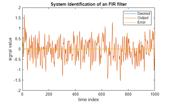
The output signal matches the desired signal, making the error between the two close to zero.
plot(1:1000, [d,y,e]);
title('System Identification of an FIR filter');
legend('Desired', 'Output', 'Error');
xlabel('time index');
ylabel('signal value');
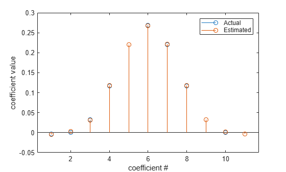
Compare the weights
The weights vector w represents the coefficients of the RLS filter that is adapted to resemble the unknown system (FIR filter). To confirm the convergence, compare the numerator of the FIR filter and the estimated weights of the RLS filter.
The estimated filter weights closely match the actual filter weights, confirming the results seen in the previous signal plot.
stem([filt.Numerator; w].');
legend('Actual','Estimated');
xlabel('coefficient #');
ylabel('coefficient value');
This example demonstrates the RLS adaptive algorithm using the inverse system identification model shown here.
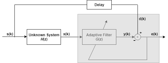
Cascading the adaptive filter with an unknown filter causes the adaptive filter to converge to a solution that is the inverse of the unknown system.
If the transfer function of the unknown system and the adaptive filter are H(z) and G(z), respectively, the error measured between the desired signal and the signal from the cascaded system reaches its minimum when G(z)H(z) = 1. For this relation to be true, G(z) must equal 1/H(z), the inverse of the transfer function of the unknown system.
To demonstrate that this is true, create a signal s to input to the cascaded filter pair.
s = randn(3000,1);
In the cascaded filters case, the unknown filter results in a delay in the signal arriving at the summation point after both filters. To prevent the adaptive filter from trying to adapt to a signal it has not yet seen (equivalent to predicting the future), delay the desired signal by 12 samples, which is the order of the unknown system.
Generally, you do not know the order of the system you are trying to identify. In that case, delay the desired signal by number of samples equal to half the order of the adaptive filter. Delaying the input requires prepending 12 zero-value samples to the input s.
delay = zeros(12,1);
d = [delay; s(1:2988)]; % Concatenate the delay and the signal.
You have to keep the desired signal vector d the same length as x, so adjust the signal element count to allow for the delay samples.
Although not generally the case, for this example you know the order of the unknown filter, so add a delay equal to the order of the unknown filter.
For the unknown system, use a lowpass, 12th-order FIR filter.
filt = dsp.FIRFilter;
filt.Numerator = designLowpassFIR(FilterOrder=12,CutoffFrequency=0.55);
Filtering s provides the input data signal for the adaptive algorithm function.
x = filt(s);
To use the RLS algorithm, create a dsp.RLSFilter object and set its Length, ForgettingFactor, and InitialInverseCovariance properties.
For more information about the input conditions to prepare the RLS algorithm object, refer to dsp.RLSFilter.
p0 = 2 * eye(13);
lambda = 0.99;
rls = dsp.RLSFilter(13,'ForgettingFactor',lambda,...
   'InitialInverseCovariance',p0);
This example seeks to develop an inverse solution, you need to be careful about which signal carries the data and which is the desired signal.
Earlier examples of adaptive filters use the filtered noise as the desired signal. In this case, the filtered noise (x) carries the unknown system's information. With Gaussian distribution and variance of 1, the unfiltered noise d is the desired signal. The code to run this adaptive filter is:
[y,e] = rls(x,d);
where y returns the filtered output and e contains the error signal as the filter adapts to find the inverse of the unknown system.
Obtain the estimated coefficients of the RLS filter.
b = rls.Coefficients;
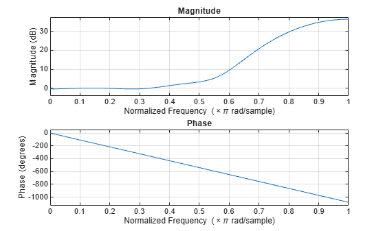
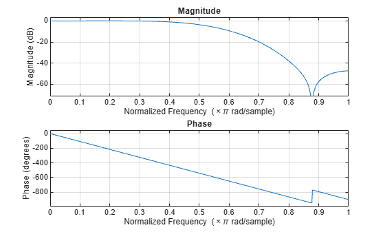
View the frequency response of the adapted RLS filter (inverse system, G(z)) using freqz. The inverse system looks like a highpass filter with linear phase.
freqz(b,1)
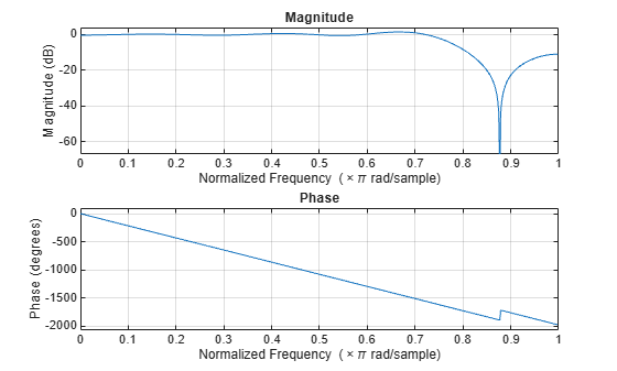
View the frequency response of the unknown system, H(z). The response is that of a lowpass filter with a cutoff frequency of 0.55.
freqz(filt.Numerator,1)
The result of the cascade of the unknown system and the adapted filter is a compensated system with an extended cutoff frequency of 0.8.
overallCoeffs = conv(filt.Numerator,b);
freqz(overallCoeffs,1)
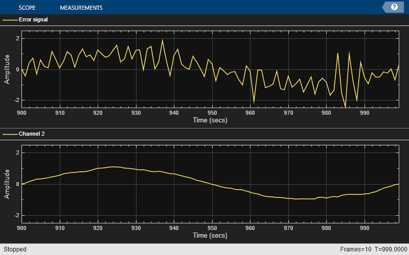
Cancel additive noise n added to an unknown system using an RLS filter. The RLS filter adapts its coefficients until its transfer function matches the transfer function of the unknown system as closely as possible. The difference between the output of the adaptive filter and the output of the unknown system is the error signal e, which represents the additive white noise. Minimizing this error signal is the objective of the adaptive filter.
Initialization
Create a dsp.FIRFilter System object™ to represent the unknown system. Create a dsp.RLSFilter object and set the length to 11 taps. Set the method to 'Householder RLS'. Create a sine wave to represent the noise added to the unknown system. View the signals in a time scope.
FrameSize = 100;
NIter = 10;

rls = dsp.RLSFilter('Length',11,...
    'Method','Householder RLS');
filt = dsp.FIRFilter('Numerator',...
    fir1(10,[.5,.75]));

sinewave = dsp.SineWave('Frequency',0.01,...
    'SampleRate',1,...
    'SamplesPerFrame',FrameSize);
scope = timescope('LayoutDimensions',[2 1],...
    'NumInputPorts',2, ...
    'TimeUnits','Seconds',...
    'YLimits',[-2.5 2.5], ...
    'BufferLength',2*FrameSize*NIter,...
    'ActiveDisplay',1,...
    'ShowLegend',true,...
    'ChannelNames',{'Noisy signal'},...
    'ActiveDisplay',2,...
    'ShowLegend',true,...
    'ChannelNames',{'Error signal'});

for k = 1:NIter
    x = randn(FrameSize,1);
    d = filt(x) + sinewave();
    [y,e] = rls(x,d);
    w = rls.Coefficients;
    scope(d,e)
end
release(scope)
Algorithms
The dsp.RLSFilter System object, when Conventional RLS is selected, recursively
computes the least squares estimate (RLS) of the FIR filter weights.
The System object estimates the filter weights or coefficients,
needed to convert the input signal into the desired signal. The input
signal can be a scalar or a column vector. The desired signal must
have the same data type, complexity, and dimensions as the input signal.
The corresponding RLS filter is expressed in matrix form as P(n)
:
where λ-1 denotes the reciprocal of the exponential weighting factor. The variables are as follows:
| Variable | Description |
|---|---|
| n | The current time index |
| u(n) | The vector of buffered input samples at step n |
| P(n) | The conjugate of the inverse correlation matrix at step n |
| k(n) | The gain vector at step n |
| k*(n) | Complex conjugate of k |
| w(n) | The vector of filter tap estimates at step n |
| y(n) | The filtered output at step n |
| e(n) | The estimation error at step n |
| d(n) | The desired response at step n |
| λ | The forgetting factor |
u, w, and k are all column vectors.
References
[1] M Hayes, Statistical Digital Signal Processing and Modeling, New York: Wiley, 1996.
[2] S. Haykin, Adaptive Filter Theory, 4th Edition, Upper Saddle River, NJ: Prentice Hall, 2002.
[3] A.A. Rontogiannis and S. Theodoridis, "Inverse factorization adaptive least-squares algorithms," Signal Processing, vol. 52, no. 1, pp. 35-47, July 1996.
[4] S.C. Douglas, "Numerically-robust O(N2) RLS algorithms using least-squares prewhitening," Proc. IEEE Int. Conf. on Acoustics, Speech, and Signal Processing, Istanbul, Turkey, vol. I, pp. 412-415, June 2000.
[5] A. H. Sayed, Fundamentals of Adaptive Filtering, Hoboken, NJ: John Wiley & Sons, 2003.
Extended Capabilities
Version History
Introduced in R2013a