Main Content

dsphdl.LMSFilter

Minimize error between observed and desired signals

Since R2023a

Description

The dsphdl.LMSFilter System object™ estimates the filter weights and minimizes the error between a desired signal and an observed signal using the mean square error (MSE) criteria. The System object adapts its weights until the error between the data and the desired data is minimal. The System object accepts scalar and vector inputs of type real and complex.

You can use this System object for various applications, such as noise cancellation, system identification, and inverse system modeling. The System object provides an architecture suitable for HDL code generation and hardware deployment. The System object provides an architecture suitable for HDL code generation and hardware deployment.

To filter input data with an LMS filter:

  1. Create the dsphdl.LMSFilter object and set its properties.

  2. Call the object with arguments, as if it were a function.

To learn more about how System objects work, see What Are System Objects?

Note

You can also generate HDL code for this hardware-optimized algorithm, without creating a MATLAB® script, by using the DSP HDL IP Designer app. The app provides the same interface and configuration options as the System object.

Creation

Description

LMSFilter = dsphdl.LMSFilter creates an LMS filter System object, LMSFilter, with default properties.

example

LMSFilter = dsphdl.LMSFilter(Name=Value) sets properties by using one or more name-value arguments. For example, FilterLength=64 sets the filter length to 64.

Properties

expand all

Unless otherwise indicated, properties are nontunable, which means you cannot change their values after calling the object. Objects lock when you call them, and the release function unlocks them.

If a property is tunable, you can change its value at any time.

For more information on changing property values, see System Design in MATLAB Using System Objects.

Specify the length of the filter as a positive integer less than or equal to 2048.

Choose how to specify the step size factor.

Specify the step size factor as a positive scalar numeric value.

Dependencies

To enable this property, set StepSizeSource to 'Property'.

Specify the initial values of the filter coefficients as a scalar or row vector of length equal to the FilterLength property value.

When you specify a scalar value, the object considers it as a row vector equivalent to the specified scalar value. The default value of this property is 0.

Enable adapt input argument of the object.

Enable weights output argument of the object.

For each iteration, the object outputs the current updated filter weights from this argument.

Enable error output argument of the object. When enabled, the object returns the result of subtracting the output signal from the desired signal.

Data Types

Rounding method for type-casting the output, specified as 'Floor', 'Ceiling', 'Convergent', 'Nearest', 'Round', or 'Zero'. The object uses this property when casting the output to the data type specified by the OutputDataType property. When the input data type is floating point, the object ignores this property. For more details, see Rounding Modes.

Overflow action, specified as 'Wrap' or 'Saturate'.

Step size data type, specified as 'Same word length as input' or '<data type expression>'.

Step size error product data type, specified as 'Full precision', 'Same word length as input', or '<data type expression>'.

Specify the filter weights fixed-point data type as one of 'Same as input', 'numerictype(1,16,15)', or '<data type expression>'.

Control Arguments

Option to enable the reset input argument, specified as true or false. When you set this property to true, the object expects a value for the reset input argument. The reset signal implements a local synchronous reset of the data path registers.

For more reset considerations, see the Reset Signal section on the Hardware Control Signals page.

Option to connect the data path registers to the generated HDL global reset signal, specified as true or false. Set this property to true to connect the generated HDL global reset signal to the data path registers. This property does not change the arguments of the object or modify simulation behavior in MATLAB. When you set this property to false, the generated HDL global reset clears only the control path registers. The generated HDL global reset can be synchronous or asynchronous depending on your HDL code generation settings.

For more reset considerations, see the Reset Signal section on the Hardware Control Signals page.

Usage

Description

[dataOut,validOut] = LMSFilt(dataIn,desiredIn,validIn) returns the LMS filtered data, dataOut, for inputs, dataIn and desiredIn, when validIn is true. validIn and validOut are logical scalars that indicate the validity of the input and output signals, respectively.

example

[dataOut,validOut,error,weights] = LMSFilt(dataIn,desiredIn,validIn,adapt) returns the LMS filtered data, dataOut and also returns error, error, and weights weights data, for inputs, dataIn, desiredIn, and adapt, when validIn is true. validIn and validOut are logical scalars that indicate the validity of the input and output signals, respectively.

To use this syntax, set the AdaptInputPort, ErrorOutputPort, and WeightsOutputPort properties to true. For example:

LMSFilt = dsphdl.LMSFilter(___,AdaptInputPort=true, ...
                               ErrorOutputPort=true, ...
                               WeightsOutputPort=true);
[dataOut,validOut,error,weights] = LMSFilt(dataIn,validIn,adapt)

example

[dataOut,validOut] = LMSFilt(dataIn,desiredIn,validIn,resetIn) returns the LMS filtered data, dataOut when validIn is true and resetIn is false. When resetIn is true, the object stops the current calculation and clears all internal state.

To use this syntax set the ResetInputPort property to true.

Input Arguments

expand all

Input data, specified as a scalar or column vector of real or complex values. The input vector size must be in the range [2, 64] and it must be less than the filter length.

You can use double and single data types for simulation, but not for HDL code generation. For HDL code generation, the input date type must be signed fixed point.

Data Types: single | double | fi
Complex Number Support: Yes

Control signal that indicates if the input data is valid. When validIn is 1 (true), the object captures the values from the input arguments dataIn and desiredIn. When validIn is 0 (false), the object ignores the values from the output arguments dataIn and desiredIn.

Data Types: logical

Desired input data, specified as a scalar or column vector of real or complex values. The input vector size must be in the range [2, 64] and it must be less than filter length. The desired signal must have the same data type, complexity, and dimensions as the input data signal.

Data Types: single | double | fi
Complex Number Support: Yes

Specify the step size to control convergence and stability of the filter. The recommended step size must be less than 1/(2 x Input power x Filter length).

You can use double and single data types for simulation, but not for HDL code generation. For HDL code generation, the input date type must be unsigned fixed point.

Dependencies

To enable this argument, set StepSizeSource to 'Property'.

Data Types: double | single | fi

When adapt is 1 (true) and validIn is 1 (true), the object adapts to the new filter weights for every validIn. When the adapt is 0 (false) and the input validIn is 1 (true) or 0 (false), the object remains at its previous filter weights.

Dependencies

To enable this argument, set AdaptInputPort to true.

Data Types: logical

Control signal that clears internal states. When resetIn is 1 (true), the object stops the current calculation, clears internal states, and sets to the initial values of filter weights specified for the InitialConditions property. When the resetIn is 0 (false) and the input validIn is 1 (true), the block captures data for processing.

For more reset considerations, see the Reset Signal section on the Hardware Control Signals page.

Dependencies

To enable this argument, set the ResetInputPort property to true.

Data Types: logical

Output Arguments

expand all

Filtered output data, returned as a scalar or column vector of real or complex values. The dimensions of the output data match the dimensions of the input data.

When the input data is a floating-point type, the output data inherits the data type of the input data. When the input data is a fixed-point type, the output data is a fixed point with word length and fractional length incremented by 1.

Data Types: fi | single | double
Complex Number Support: Yes

Control signal that indicates if the output data is valid. When validOut is 1 (true), the object returns valid data from the dataOut argument. When validOut is 0 (false), values from the dataOut argument are not valid.

Data Types: logical

Outputs the result of subtracting the filtered output signal from the desired signal when the output argument validOut is 1 (true).

If the input data and desired is a scalar or a column vector, the error signal has the same dimension and complexity as the input data. When the input data is a floating-point type, the output data inherits the data type of the input data. When the input data is a fixed-point type, the output data is fixed point with word length incremented by 2 and fractional length incremented by 1.

Dependencies

To enable this argument, set ErrorOutputPort to true.

Data Types: logical

For each iteration, the object outputs the current updated filter weights from this argument when the output argument validOut is 1 (true).

For floating-point inputs, the weights data type must match the input type. For fixed-point signals, the input must match the data type set to the WeightsDataType property.

Dependencies

To enable this argument, set WeightsOutputPort to true.

Data Types: logical

Object Functions

To use an object function, specify the System object as the first input argument. For example, to release system resources of a System object named obj, use this syntax:

release(obj)

expand all

getLatencyLatency of LMS Filter
stepRun System object algorithm
releaseRelease resources and allow changes to System object property values and input characteristics
resetReset internal states of System object

Examples

collapse all

This example shows how use the dsphdl.LMSFilter System object™ for system identification. System identification is a process to identify the coefficients of an unknown system using an adaptive filter. For more information, see System Identification –– Using an Adaptive Filter to Identify an Unknown System.

Set Up Input Parameters

Set up input variables for the System object dsphdl.LMSFilter and the reference System object dsp.LMSFilter to use.

filterLength = 35;
stepSize = 0.008;
frameSize = 1500;

Initialize System Objects

Initialize the dsphdl.LMSFilter System object and the reference System object dsphdl.LMSFilter with the required properties.

HDLLMSFilterObj = dsphdl.LMSFilter(FilterLength=filterLength, ...
    StepSize=stepSize, ...
    WeightsOutputPort=true, ...
    ErrorOutputPort=true);
% dsp.LMSFilter for reference
lmsfilt = dsp.LMSFilter(filterLength,StepSize=stepSize);

Design System Parameters for Indentification

Create a dsp.FIRFilter object that represents a system to be identified. Use fir1 function to design the filter coefficients. The designed filter is a lowpass filter with 0.25 cut-off frequency.

b = fir1(filterLength-1,0.25); % channel coefficients
firfilt1 = dsp.FIRFilter(b); % filter object

% Initialize array plot function
AP = dsp.ArrayPlot(YLimits=[-0.1 .3], ...
    ShowLegend=true, ...
    Position=[0 0 560 420], ...
    ChannelNames={'Actual Coefficients', ...
    'dsphdl.LMSFilter Estimated Coefficients', ...
    'dsp.LMSFilter Estimated Coefficients'});

Generate Input Observed and Desired Signals

Use randn function to generate observed input signal x and AWGN noise signal n. Apply the firfilt1 function on the signal x. Add the signal n to x and generate the desired signal d. Provide these signals as input to the LMS filter System objects and capture their outputs.

x = fi(randn(frameSize,1),1,16,13);   % input observed signal
n = 0.001*randn(frameSize,1);         % AWGN noise signal
d = fi(firfilt1(x) + n ,1,16,13);     % input desired signal

% Initialize intermediate variables
y = zeros(length(x),1);
e = zeros(length(x),1);
w = zeros(length(x),filterLength);
v = zeros(length(x),1);
for ii=1:length(x)
    [ y(ii,:), v(ii,:), e(ii,:), w(ii,:)] = ...
        HDLLMSFilterObj(x(ii), d(ii), true );
end

% Capture valid output data
y = y(v==1,:); % filter output
w = w(v==1,:); % filter weights output
e = e(v==1,:); % filter error output

% Capture reference output
[y1,e1,w1] = lmsfilt(double(x),double(d));

Compare Output Weights

The weight vectors w and w1 represent the weights of the LMS filter object dsphdl.LMSFilter and the reference object dsp.LMSFilter, respectively. To confirm the convergence, compare the numerator of the design system firfilt1 with the estimated weights of the LMS filter System object dsphdl.LMSFilter and the reference System object dsp.LMSFilter.

% Plot numerators |b|, |w|, and |w1|.
AP([b.',double(w(end,:)).',w1(:)]);

The latency of the dsphdl.LMSFilter System object™ varies with the input size and filter length. Use the getLatency function to find the latency of an LMS Filter for a particular configuration. The latency is measured as the number of cycles between the first valid input and the first valid output, assuming that the input is contiguous.

Create dsphdl.LMSFilter System object and calculate latency.

lmsfilter = dsphdl.LMSFilter
lmsfilter = 
  dsphdl.LMSFilter with properties:

         FilterLength: 32
       StepSizeSource: 'Property'
             StepSize: 0.0100
    InitialConditions: 0
       AdaptInputPort: false
    WeightsOutputPort: true
      ErrorOutputPort: false

  Use get to show all properties

Calculate latency for the object with a filter length 64.

lmsfilter = dsphdl.LMSFilter(FilterLength=64);
latencyDT = getLatency(lmsfilter)
latencyDT = 
13

Calculate latency for the object with a filter length 75. The latency does not change.

lmsfilter = dsphdl.LMSFilter(FilterLength=75);
latencyDT = getLatency(lmsfilter)
latencyDT = 
13

Calculate latency when the input is complex.

latencyDT = getLatency(lmsfilter,complex(0))
latencyDT = 
15

Calculate latency when input is real with vector size 4.

latencyDT = getLatency(lmsfilter,real(0),4)
latencyDT = 
18

Algorithms

expand all

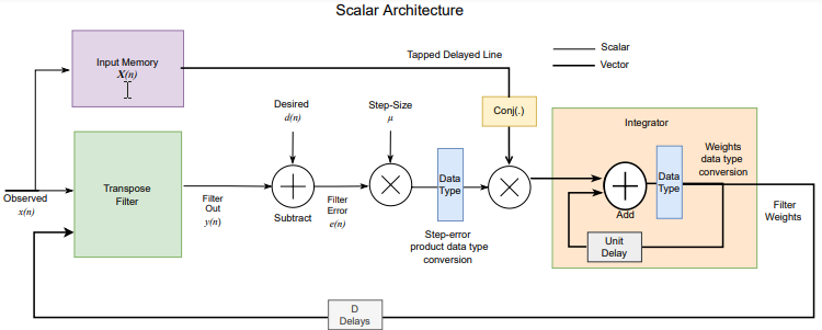
The following figure shows the high-level architecture block diagram of the LMS Filter System object for a scalar input. An observed signal is provided as input to the Input Memory block and also to the Transpose Filter block, which is configured with a Discrete FIR Filter block. The output of the Transpose Filter block is subtracted from the Desired input signal to output the Filter Error signal. The Filter Error signal is multiplied with the Step-Size input signal and the resulted step-error product converted to the required data type. The step-error product is multiplied with the corresponding tap delay line conjugate from the Input Memory block. In the Integrator block, the multiplied output is added to the previous weight, Unit Delay, to output new filter weights. These filter weights are routed back to the Transpose Filter block for the next weight updates.

LMS Filter scalar architecture

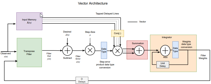
The following figure shows the high-level architecture block diagram of the LMS Filter System object for vector input. The vector architecture is almost similar to the scalar architecture. In the vector architecture, step-error product vectors are multiplied with the corresponding tap delay line conjugates from the Input Memory block and then summed up in the Summation block. In the Integrator block, the summed output is added to the previous weight vector Unit Delay to output new filter weights. These filter weights are routed back to the Transpose Filter block for the next weight updates.

LMS Filter vector architecture

For hardware implementation, all these operations are pipelined, which takes around D number of delays to update the filter weights, where D is the latency of the System object.

References

[1] Hayes, M.H. Statistical Digital Signal Processing and Modeling. New York: John Wiley & Sons, 1996.

Extended Capabilities

Version History

Introduced in R2023a

See Also

Blocks

Go to top of page