Main Content

dsp.FastTransversalFilter

Fast transversal least-squares FIR adaptive filter

Description

The dsp.FastTransversalFilter computes output, error and coefficients using a fast transversal least-squares FIR adaptive filter.

To implement the adaptive FIR filter object:

  1. Create the dsp.FastTransversalFilter object and set its properties.

  2. Call the object with arguments, as if it were a function.

To learn more about how System objects work, see What Are System Objects?

Creation

Description

ftf = dsp.FastTransversalFilter returns a System object™, ftf, which is a fast transversal, least-squares FIR adaptive filter. This System object computes the filtered output and the filter error for a given input and desired signal.

example

ftf = dsp.FastTransversalFilter(len) returns a dsp.FastTrasversalFilter System object with the Length property set to len.

ftf = dsp.FastTransversalFilter(Name,Value) returns a dsp.FastTransversalFilter System object with each specified property set to the specified value.

Properties

expand all

Unless otherwise indicated, properties are nontunable, which means you cannot change their values after calling the object. Objects lock when you call them, and the release function unlocks them.

If a property is tunable, you can change its value at any time.

For more information on changing property values, see System Design in MATLAB Using System Objects.

Specify the method used to calculate filter coefficients as either 'Fast transversal least-squares' or 'Sliding-window fast transversal least-squares'. For algorithms used to implement these two different methods, refer to [1]. This property is nontunable.

Specify the length of the FIR filter coefficients vector as a positive integer value.

Data Types: double

Specify the width of the sliding window as a positive integer value greater than or equal to the Length property value. The default vale is the value of the Length property.

Dependencies

This property applies only if the Method property is set to 'Sliding-window fast transversal least-squares'.

Data Types: double

Specify the fast transversal filter forgetting factor as a positive scalar in the range (0,1]. Setting this value to 1 denotes infinite memory while filter adaptation. Setting this property value to 1 denotes infinite memory while adapting to find the new filter. For best results, set this property to a value that lies in the range [1-0.5/L,1], where L is the Length property value.

Tunable: Yes

Dependencies

This property applies only if the Method property is set to 'Fast transversal least-squares'.

Data Types: single | double | int8 | int16 | int32 | int64 | uint8 | uint16 | uint32 | uint64 | logical

Specify the initial value of the forward and backward prediction error vectors as a positive numeric scalar. This scalar should be sufficiently large to maintain stability and prevent an excessive number of Kalman gain rescues.

Tunable: Yes

Data Types: single | double | int8 | int16 | int32 | int64 | uint8 | uint16 | uint32 | uint64

Specify the initial value of the conversion factor of the fast transversal filter.

The value of this property depends on the Method property. If Method is set to:

  • 'Fast transversal least-squares' –– This property must be a positive numeric value less than or equal to 1

  • 'Sliding-window fast transversal least-squares' –– This property must be a two-element numeric vector. The first element of this vector must lie within the range [0,1], and the second element must be less than or equal to -1. In this case, the default value is [1,-1].

Tunable: Yes

Data Types: single | double | int8 | int16 | int32 | int64 | uint8 | uint16 | uint32 | uint64 | logical

Specify the initial values of the FIR adaptive filter coefficients as a scalar or a vector of length equal to the value of the Length property.

Tunable: Yes

Data Types: single | double | int8 | int16 | int32 | int64 | uint8 | uint16 | uint32 | uint64

Specify whether to lock the filter coefficient values. By default, the value of this property is false, and the object continuously updates the filter coefficients. If this property is set to true, the filter coefficients do not update, and their values remain the same.

Tunable: Yes

Usage

Description

example

[y,err] = ftf(x,d) filters the input x, using d as the desired signal, and returns the filtered output in y and the filter error in err. The System object estimates the filter weights needed to minimize the error between the output signal and the desired signal.

Input Arguments

expand all

The signal to be filtered by the fast transversal filter. The input, x, and the desired signal, d must have the same size and data type.

The data input can be a variable-size signal. You can change the number of elements in the column vector even when the object is locked. The System object locks when you call the object to run its algorithm.

Data Types: single | double
Complex Number Support: Yes

The fast transversal filter adapts its filter weights, wts, to minimize the error, err, and converge the input signal x to the desired signal d as closely as possible. You can access the current filter weights by calling ftf.Coefficients, where ftf is the fast transversal filter object.

The input and the desired signal must have the same size and data type.

The desired signal can be a variable-size signal. You can change the number of elements in the column vector even when the object is locked. The System object locks when you call the object to run its algorithm.

Data Types: single | double
Complex Number Support: Yes

Output Arguments

expand all

Filtered output, returned as a scalar or a column vector. The object adapts its filter weights to converge the input signal x to match the desired signal d. The filter outputs the converged signal.

Data Types: single | double

Difference between the output signal y and the desired signal d, returned as a scalar or a column vector. The data type of err matches the data type of y. The objective of the adaptive filter is to minimize this error. The object adapts its weights to converge toward optimal filter weights that produce an output signal that matches closely with the desired signal.

Data Types: single | double

Object Functions

To use an object function, specify the System object as the first input argument. For example, to release system resources of a System object named obj, use this syntax:

release(obj)

expand all

msesimEstimated mean squared error for adaptive filters
stepRun System object algorithm
releaseRelease resources and allow changes to System object property values and input characteristics
resetReset internal states of System object

Examples

collapse all

System identification is the process of identifying the coefficients of an unknown system using an adaptive filter. The general overview of the process is shown in System Identification –– Using an Adaptive Filter to Identify an Unknown System. The main components involved are:

  • The adaptive filter algorithm.

  • An unknown system or process to adapt to. In this example, the filter designed by designLowpassFIR is the unknown system.

  • Appropriate input data to exercise the adaptation process. In a generic system identification model, the desired signal d(k) and the input signal x(k) are used to exercise the adaptation process.

The objective of the adaptive filter is to minimize the error signal between the output of the adaptive filter y(k) and the output of the unknown system (or the system to be identified) d(k). Once the error signal is minimized, the adapted filter resembles the unknown system. The coefficients of both the filters match closely.

Unknown System

Create a dsp.FIRFilter object that represents the system to be identified. Use the designLowpassFIR function to design the filter coefficients. The designed filter is a 10th order lowpass digital filter with a cutoff frequency of 0.25.

filt = dsp.FIRFilter;
filt.Numerator = designLowpassFIR(FilterOrder=10,CutoffFrequency=.25)
filt = 
  dsp.FIRFilter with properties:

            Structure: 'Direct form'
      NumeratorSource: 'Property'
            Numerator: [-0.0039 1.7585e-18 0.0321 0.1167 0.2207 0.2687 0.2207 0.1167 0.0321 1.7585e-18 -0.0039]
    InitialConditions: 0

  Use get to show all properties

Pass the signal x to the FIR filter. The desired signal d is the sum of the output of the unknown system (FIR filter) and an additive noise signal n.

x = randn(1000,1);
d = filt(x) + 0.01*randn(1000,1);

Adaptive Filter

With the unknown filter designed and the desired signal in place, create and apply the fast transversal filter object to identify the unknown filter.

Create a dsp.FastTransversalFilter object to represent an adaptive filter. Set the length of the adaptive filter to 11 taps and a forgetting factor of 0.99.

ftf1 = dsp.FastTransversalFilter(11,...
    'ForgettingFactor',0.99)
ftf1 = 
  dsp.FastTransversalFilter with properties:

                         Method: 'Fast transversal least-squares'
                         Length: 11
               ForgettingFactor: 0.9900
    InitialPredictionErrorPower: 10
            InitialCoefficients: 0
        InitialConversionFactor: 1
               LockCoefficients: false

Pass the primary input signal x and the desired signal d to the fast transversal filter. Run the adaptive filter to determine the unknown system. The output y of the adaptive filter is the signal converged to the desired signal d, thereby minimizing the error e between the two signals.

[y,e] = ftf1(x,d);
w = ftf1.Coefficients
w = 1×11

   -0.0043    0.0016    0.0308    0.1171    0.2204    0.2677    0.2210    0.1181    0.0323    0.0013   -0.0037

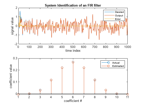
Plot the results. The output signal matches the desired signal very closely making the error between the two close to zero.

subplot(2,1,1);
plot(1:1000,[d,y,e])
title('System Identification of an FIR filter');
legend('Desired','Output','Error');
xlabel('time index');
ylabel('signal value');

The coefficients of the FIR filter match very closely with the coefficients of the adapted filter, thereby confirming the convergence.

subplot(2,1,2); 
stem([filt.Numerator; w].');
legend('Actual','Estimated'); 
xlabel('coefficient #'); 
ylabel('coefficient value');

References

[1] Haykin, Simon. Adaptive Filter Theory, 4th Ed. Upper Saddle River, NJ: Prentice Hall, 2002.

Extended Capabilities

Version History

Introduced in R2013b