Main Content

dsp.AdaptiveLatticeFilter

Adaptive lattice filter

Description

The dsp.AdaptiveLatticeFilter System object™ computes output, error, and coefficients using a lattice-based FIR adaptive filter.

To implement the adaptive FIR filter object:

  1. Create the dsp.AdaptiveLatticeFilter object and set its properties.

  2. Call the object with arguments, as if it were a function.

To learn more about how System objects work, see What Are System Objects?

Creation

Description

alf = dsp.AdaptiveLatticeFilter returns a lattice-based FIR adaptive filter System object, alf. This System object computes the filtered output and the filter error for a given input and desired signal.

example

alf = dsp.AdaptiveLatticeFilter(len) returns an AdaptiveLatticeFilter System object with the Length property set to len.

example

alf = dsp.AdaptiveLatticeFilter(Name,Value) returns an AdaptiveLatticeFilter System object with each specified property set to the specified value. Enclose each property name in single quotes. Unspecified properties have default values.

Properties

expand all

Unless otherwise indicated, properties are nontunable, which means you cannot change their values after calling the object. Objects lock when you call them, and the release function unlocks them.

If a property is tunable, you can change its value at any time.

For more information on changing property values, see System Design in MATLAB Using System Objects.

Specify the method used to calculate filter coefficients as one of 'Least-squares Lattice', 'QR-decomposition Least-squares Lattice', 'Gradient Adaptive Lattice'. The default value is 'Least-squares Lattice'. For algorithms used to implement these three different methods, refer to [1] [2]. This property is nontunable.

Specify the length of the FIR filter coefficients vector as a positive integer value. This property is nontunable.

Data Types: single | double | int8 | int16 | int32 | int64 | uint8 | uint16 | uint32 | uint64

Specify the least-squares lattice forgetting factor as a scalar positive numeric value less than or equal to 1. Setting this value to 1 denotes infinite memory during adaptation.

Tunable: Yes

Dependencies

This property applies only if the Method property is set to 'Least-squares Lattice' or 'QR-decomposition Least-squares Lattice'.

Data Types: single | double | int8 | int16 | int32 | int64 | uint8 | uint16 | uint32 | uint64

Specify the joint process step size of the gradient adaptive lattice filter as a positive numeric scalar less than or equal to 1.

Tunable: Yes

Dependencies

This property applies only if the Method property is set to 'Gradient Adaptive Lattice'.

Data Types: single | double | int8 | int16 | int32 | int64 | uint8 | uint16 | uint32 | uint64 | logical

Specify an offset value for the denominator of the StepSize normalization term as a nonnegative numeric scalar. A nonzero offset helps avoid a divide-by-near-zero condition when the input signal amplitude is very small.

Tunable: Yes

Dependencies

This property applies only if the Method property is set to 'Gradient Adaptive Lattice'.

Data Types: single | double | int8 | int16 | int32 | int64 | uint8 | uint16 | uint32 | uint64

Specify the reflection process step size of the gradient adaptive lattice filter as a scalar numeric value between 0 and 1, both inclusive. The default value is the StepSize property value.

Tunable: Yes

Dependencies

Use this property only if the Method property is set to 'Gradient Adaptive Lattice'.

Data Types: single | double | int8 | int16 | int32 | int64 | uint8 | uint16 | uint32 | uint64 | logical

Specify the averaging factor as a positive numeric scalar less than 1. Use this property to compute the exponentially windowed forward and backward prediction error powers for the coefficient updates. The default is the value of 1 - StepSize.

Tunable: Yes

Dependencies

This property applies only if the Method property is set to'Gradient Adaptive Lattice.

Data Types: single | double

Specify the initial values for the prediction error vectors as a scalar positive numeric value.

If the Method property is set to 'Least-squares Lattice' or 'QR-decomposition Least-squares Lattice', the default value is 1.0. If the Method property is set to 'Gradient Adaptive Lattice', the default value is 0.1.

Tunable: Yes

Data Types: single | double

Specify the initial values of the FIR adaptive filter coefficients as a scalar or a vector of length equal to the value of the Length property.

Tunable: Yes

Data Types: single | double | int8 | int16 | int32 | int64 | uint8 | uint16 | uint32 | uint64

Specify whether to lock the filter coefficient values. By default, the value of this property is false, and the object continuously updates the filter coefficients. If this property is set to true, the filter coefficients do not update and their values remain the same.

Tunable: Yes

Dependencies

This property is applicable only if the Method property is set to 'Gradient Adaptive Lattice'.

Usage

Description

example

[y,err] = alf(x,d) filters the input x, using d as the desired signal, and returns the filtered output in y and the filter error in err. The System object estimates the filter weights needed to minimize the error between the output signal and the desired signal. You can access these coefficients by accessing the Coefficients property of the object. This can be done only after calling the object. For example, to access the optimized coefficients of the alf filter, call alf.Coefficients after you pass the input and desired signal to the object.

Input Arguments

expand all

The signal to be filtered by the adaptive lattice filter. The input, x, and the desired signal, d, must have the same size and data type.

The input can be a variable-size signal. You can change the number of elements in the column vector even when the object is locked. The System object locks when you call the object.

Data Types: single | double
Complex Number Support: Yes

The adaptive lattice filter adapts its coefficients to minimize the error, err, and converge the input signal x to the desired signal d as closely as possible.

The input, x, and the desired signal, d, must have the same size and data type.

The desired signal can be a variable-size signal. You can change the number of elements in the column vector even when the object is locked. The System object locks when you call the object.

Data Types: single | double
Complex Number Support: Yes

Output Arguments

expand all

Filtered output, returned as a scalar or a column vector. The object adapts its filter coefficients to converge the input signal x to match the desired signal d. The filter outputs the converged signal.

Data Types: single | double
Complex Number Support: Yes

Difference between the output signal y and the desired signal d, returned as a scalar or a column vector. The objective of the adaptive lattice filter is to minimize this error. The object adapts its coefficients to converge towards optimal filter coefficients that produce an output signal that matches closely with the desired signal. To access the adaptive lattice filter coefficients, call alf.Coefficients after you pass the input and desired signal to the object algorithm.

Data Types: single | double
Complex Number Support: Yes

Object Functions

To use an object function, specify the System object as the first input argument. For example, to release system resources of a System object named obj, use this syntax:

release(obj)

expand all

msesimEstimated mean squared error for adaptive filters
stepRun System object algorithm
releaseRelease resources and allow changes to System object property values and input characteristics
resetReset internal states of System object

Examples

collapse all

Create the QPSK signal and the noise, filter them to obtain the received signal, and delay the received signal to obtain the desired signal.

D = 16;
b = exp(1i*pi/4)*[-0.7 1];
a = [1 -0.7];
ntr = 1000;
s = sign(randn(1,ntr+D)) + 1i*sign(randn(1,ntr+D));
n = 0.1*(randn(1,ntr+D) + 1i*randn(1,ntr+D));
r = filter(b,a,s) + n;
x = r(1+D:ntr+D);
d = s(1:ntr);

Use the Adaptive Lattice Filter to compute the filtered output and the filter error for the input and desired signal.

lam = 0.995;
del = 1;
alf = dsp.AdaptiveLatticeFilter('Length', 32, ...
    'ForgettingFactor', lam, 'InitialPredictionErrorPower', del);
[y,e] = alf(x,d);

Plot the In-Phase and the Quadrature components of the desired, output, and the error signals.

subplot(2,2,1); plot(1:ntr,real([d;y;e]));
title('In-Phase Components');
legend('Desired','Output','Error');
xlabel('time index'); ylabel('signal value');
subplot(2,2,2); plot(1:ntr,imag([d;y;e]));
title('Quadrature Components');
legend('Desired','Output','Error');
xlabel('time index'); ylabel('signal value');

Figure contains 2 axes objects. Axes object 1 with title In-Phase Components, xlabel time index, ylabel signal value contains 3 objects of type line. These objects represent Desired, Output, Error. Axes object 2 with title Quadrature Components, xlabel time index, ylabel signal value contains 3 objects of type line. These objects represent Desired, Output, Error.

Plot the received and equalized signals’ scatter plots.

subplot(2,2,3); plot(x(ntr-100:ntr),'.'); axis([-3 3 -3 3]);
title('Received Signal Scatter Plot'); axis('square'); 
xlabel('Real[x]'); ylabel('Imag[x]'); grid on;
subplot(2,2,4); plot(y(ntr-100:ntr),'.'); axis([-3 3 -3 3]);
title('Equalized Signal Scatter Plot'); axis('square');
xlabel('Real[y]'); ylabel('Imag[y]'); grid on;

Figure contains 4 axes objects. Axes object 1 with title In-Phase Components, xlabel time index, ylabel signal value contains 3 objects of type line. These objects represent Desired, Output, Error. Axes object 2 with title Quadrature Components, xlabel time index, ylabel signal value contains 3 objects of type line. These objects represent Desired, Output, Error. axes object 3 with title Received Signal Scatter Plot, xlabel Real[x], ylabel Imag[x] contains a line object which displays its values using only markers. axes object 4 with title Equalized Signal Scatter Plot, xlabel Real[y], ylabel Imag[y] contains a line object which displays its values using only markers.

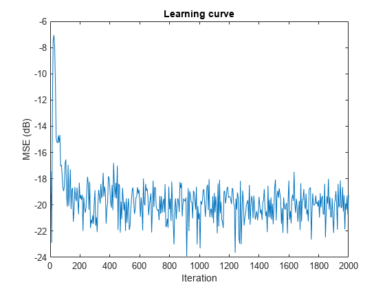
ha = fir1(31,0.5);
% FIR system to be identified 
fir = dsp.FIRFilter('Numerator',ha); 
iir = dsp.IIRFilter('Numerator',sqrt(0.75),...
        'Denominator',[1 -0.5]);
x = iir(sign(randn(2000,25))); 
% Observation noise signal 
n = 0.1*randn(size(x)); 
 % Desired signal 
d = fir(x)+n;
% Filter length 
l = 32;
% Decimation factor for analysis
% and simulation results 
m  = 5;                             
ha = dsp.AdaptiveLatticeFilter(l); 
[simmse,meanWsim,Wsim,traceKsim] = msesim(ha,x,d,m);
plot(m*(1:length(simmse)),10*log10(simmse));
xlabel('Iteration'); 
ylabel('MSE (dB)');
% Plot the learning curve used for 
% adaptive lattice filter used in system identification
title('Learning curve')

Figure contains an axes object. The axes object with title Learning curve, xlabel Iteration, ylabel MSE (dB) contains an object of type line.

References

[1] Griffiths, Lloyd J. “A Continuously Adaptive Filter Implemented as a Lattice Structure”. Proceedings of IEEE Int. Conf. on Acoustics, Speech, and Signal Processing, Hartford, CT, pp. 683–686, 1977 .

[2] Haykin, S. Adaptive Filter Theory, 4th Ed. Upper Saddle River, NJ: Prentice Hall, 1996.

Extended Capabilities

Version History

Introduced in R2013b