nlarx
Estimate parameters of nonlinear ARX model
Syntax
Description
Estimate New Nonlinear ARX Model
sys = nlarx(data,orders)data using the specified ARX model orders
orders and the default wavelet network output function.
data can be in the form of a timetable, a comma-separated pair
of numeric matrices, a single numeric matrix, or an iddata object. If
data is a timetable, you can select specific input and
output channels to use for estimation by specifying the channel names in the
InputName and OutputName
name-value arguments.
Use this syntax when you extend an ARX linear model, or when you use only regressors that are linear with consecutive lags.
sys = nlarx(data,regressors)regressors.
Use this syntax when you have linear regressors that have nonconsecutive lags, or when you also have any combination of polynomial regressors, periodic regressors, and custom regressors.
When you use regressors to estimate a MIMO system and
data is a timetable, you must also specify the output
variables in the OutputName name-value argument.
sys = nlarx(___,output_fcn)
Extend Existing Linear Model
sys = nlarx(data,linmodel)linmodel to specify the model orders
and the initial values of the linear coefficients of the model.
Use this syntax when you want to create a nonlinear ARX model as an extension of, or an improvement upon, an existing linear model.
When you use this syntax, the software initializes the offset value to
0. In some cases, you can improve the estimation results
by overriding this initialization with the command
sys.OutputFcn.Offset.Value = NaN.
sys = nlarx(data,linmodel,output_fcn)
Refine Existing Nonlinear ARX Model
sys = nlarx(data,sys0)sys0.
Use this syntax to:
Estimate the parameters of a model previously created using the
idnlarxconstructor. Prior to estimation, you can configure the model properties using dot notation.Update the parameters of a previously estimated model to improve the fit to the estimation data. In this case, the estimation algorithm uses the parameters of
sys0as initial guesses.
Specify Additional Options
sys = nlarx(___,Name,Value)sys =
nlarx(data,regressors,'InputName',["u1","u3"],'OutputName',["y1","y4"]).
Examples
Load the estimation data.
load twotankdata;Create an iddata object from the estimation data with a sample time of 0.2 seconds.
Ts = 0.2;
z = iddata(y,u,Ts);
Estimate the nonlinear ARX model using ARX model orders to specify the regressors.
sysNL = nlarx(z,[4 4 1])
sysNL =

Nonlinear ARX model with 1 output and 1 input
  Inputs: u1
  Outputs: y1

Regressors:
  Linear regressors in variables y1, u1
  List of all regressors

Output function: Wavelet network with 11 units
Sample time: 0.2 seconds

Status:
Estimated using NLARX on time domain data "z".
Fit to estimation data: 96.84% (prediction focus)
FPE: 3.482e-05, MSE: 3.431e-05

Model Properties
sys uses the default idWaveletNetwork function as the output function.
For comparison, compute a linear ARX model with the same model orders.
sysL = arx(z,[4 4 1]);
Compare the model outputs with the original data.
compare(z,sysNL,sysL)
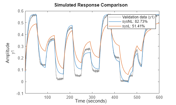
The nonlinear model has a much better fit to the data than the linear model.
Specify a linear regressor that is equivalent to an ARX model order matrix of [4 4 1].
An order matrix of [4 4 1] specifies that both input and output regressor sets contain four regressors with lags ranging from 1 to 4. For example, represents the second input regressor.
Specify the output and input names.
output_name = 'y1';
input_name = 'u1';
names = {output_name,input_name};
Specify the output and input lags.
output_lag = [1 2 3 4];
input_lag = [1 2 3 4];
lags = {output_lag,input_lag};
Create the linear regressor object.
lreg = linearRegressor(names,lags)
lreg =
Linear regressors in variables y1, u1
       Variables: {'y1'  'u1'}
            Lags: {[1 2 3 4]  [1 2 3 4]}
     UseAbsolute: [0 0]
    TimeVariable: 't'

  Regressors described by this set
Load the estimation data and create an iddata object.
load twotankdata
z = iddata(y,u,0.2);
Estimate the nonlinear ARX model.
sys = nlarx(z,lreg)
sys =

Nonlinear ARX model with 1 output and 1 input
  Inputs: u1
  Outputs: y1

Regressors:
  Linear regressors in variables y1, u1
  List of all regressors

Output function: Wavelet network with 11 units
Sample time: 0.2 seconds

Status:
Estimated using NLARX on time domain data "z".
Fit to estimation data: 96.84% (prediction focus)
FPE: 3.482e-05, MSE: 3.431e-05

Model Properties
View the regressors.
getreg(sys)
ans = 8×1 cell
    {'y1(t-1)'}
    {'y1(t-2)'}
    {'y1(t-3)'}
    {'y1(t-4)'}
    {'u1(t-1)'}
    {'u1(t-2)'}
    {'u1(t-3)'}
    {'u1(t-4)'}
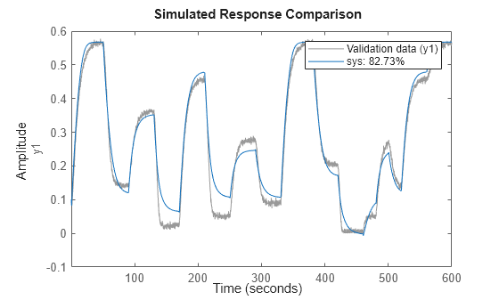
Compare the model output to the estimation data.
compare(z,sys)
Create time and data arrays.
dt = 0.01;
t = 0:dt:10;
y = 10*sin(2*pi*t)+rand(size(t));
Create an iddata object with no input signal specified.
z = iddata(y',[],dt);
Estimate the nonlinear ARX model.
sys = nlarx(z,2)
sys =

Nonlinear time series model
  Outputs: y1

Regressors:
  Linear regressors in variables y1
  List of all regressors

Output function: Wavelet network with 8 units
Sample time: 0.01 seconds

Status:
Estimated using NLARX on time domain data "z".
Fit to estimation data: 92.92% (prediction focus)
FPE: 0.2568, MSE: 0.2507

Model Properties
Estimate a nonlinear ARX model that uses the mapping function idSigmoidNetwork as its output function.
Load the data and divide it into the estimation and validation data sets ze and zv.
load twotankdata.mat u y
z = iddata(y,u,'Ts',0.2);
ze = z(1:1500);
zv = z(1501:end);
Configure the idSigmoidNetwork mapping function. Fix the offset to 0.2 and the number of units to 15.
s = idSigmoidNetwork;
s.Offset.Value = 0.2;
s. NonlinearFcn.NumberOfUnits = 15;
Create a linear model regressor specification that contains four output regressors and five input regressors.
reg1 = linearRegressor({'y1','u1'},{1:4,0:4});Create a polynomial model regressor specification that contains the squares of two output terms and three input terms.
reg2 = polynomialRegressor({'y1','u1'},{1:2,0:2},2);Set estimation options for the search method and maximum number of iterations.
opt = nlarxOptions('SearchMethod','fmincon')';
opt.SearchOptions.MaxIterations = 40;
Estimate the nonlinear ARX model.
sys = nlarx(ze,[reg1;reg2],s,opt);
Validate sys by comparing the simulated model response to the validation data set.
compare(zv,sys)

Estimate a linear model and improve the model by adding an idTreePartition output function.
Load the estimation data.
load throttledata ThrottleData
Estimate a linear ARX model linsys with orders [2 2 1].
linsys = arx(ThrottleData,[2 2 1]);
Create an idnlarx template model that uses linsys and specifies idTreePartition as the output function.
sys0 = idnlarx(linsys,idTreePartition);
Fix the linear component of sys0 so that during estimation, the linear portion of sys0 remains identical to linsys. Set the offset component value to NaN.
sys0.OutputFcn.LinearFcn.Free = false;
sys0.OutputFcn.Offset.Value = NaN;
Estimate the free parameters of sys0, which are the nonlinear-function parameters and the offset.
sys = nlarx(ThrottleData,sys0);
Compare the fit accuracies for the linear and nonlinear models.
compare(ThrottleData,linsys,sys)

Generating a custom network mapping object requires the definition of a user-defined unit function.
Define the unit function and save it as gaussunit.m.
function [f,g,a] = gaussunit(x)
% Custom unit function nonlinearity.
%
% Copyright 2015 The MathWorks, Inc.
f = exp(-x.*x);
if nargout>1
  g = -2*x.*f;
  a = 0.2;
end
Create a custom network mapping object using a handle to the gaussunit function.
H = @gaussunit;
CNet = idCustomNetwork(H);
Load the estimation data.
load iddata1
Estimate a nonlinear ARX model using the custom network.
sys = nlarx(z1,[1 2 1],CNet)
sys =

<strong>Nonlinear ARX model with 1 output and 1 input</strong>
  Inputs: u1
  Outputs: y1

Regressors:
  Linear regressors in variables y1, u1

Output function: Custom Network with 10 units and "gaussunit" unit function
Sample time: 0.1 seconds

Status:
Estimated using NLARX on time domain data "z1".
Fit to estimation data: 64.35% (prediction focus)
FPE: 3.58, MSE: 2.465
Load the estimation data.
load motorizedcamera;Create an iddata object.
z = iddata(y,u,0.02,'Name','Motorized Camera','TimeUnit','s');
z is an iddata object with six inputs and two outputs.
Specify the model orders.
Orders = [ones(2,2),2*ones(2,6),ones(2,6)];
Specify different mapping functions for each output channel.
NL = [idWaveletNetwork(2),idLinear];
Estimate the nonlinear ARX model.
sys = nlarx(z,Orders,NL)
sys =

Nonlinear ARX model with 2 outputs and 6 inputs
  Inputs: u1, u2, u3, u4, u5, u6
  Outputs: y1, y2

Regressors:
  Linear regressors in variables y1, y2, u1, u2, u3, u4, u5, u6
  List of all regressors

Output functions:
  Output 1:  Wavelet network with 2 units
  Output 2:  Linear with offset

Sample time: 0.02 seconds

Status:
Estimated using NLARX on time domain data "Motorized Camera".
Fit to estimation data: [98.82;98.77]% (prediction focus)
FPE: 0.4839, MSE: 0.9762

Model Properties
Load the estimation data and create an iddata object z. z contains two output channels and six input channels.
load motorizedcamera;
z = iddata(y,u,0.02);
Specify a set of linear regressors that uses the output and input names from z and contains:
2 output regressors with 1 lag.
6 input regressor pairs with 1 and 2 lags.
names = [z.OutputName; z.InputName];
lags = {1,1,[1,2],[1,2],[1,2],[1,2],[1,2],[1,2]};
reg = linearRegressor(names,lags);
Estimate a nonlinear ARX model using an idSigmoidNetwork mapping function with four units for all output channels.
sys = nlarx(z,reg,idSigmoidNetwork(4))
sys =

Nonlinear ARX model with 2 outputs and 6 inputs
  Inputs: u1, u2, u3, u4, u5, u6
  Outputs: y1, y2

Regressors:
  Linear regressors in variables y1, y2, u1, u2, u3, u4, u5, u6
  List of all regressors

Output functions:
  Output 1:  Sigmoid network with 4 units
  Output 2:  Sigmoid network with 4 units

Sample time: 0.02 seconds

Status:
Estimated using NLARX on time domain data "z".
Fit to estimation data: [98.86;98.79]% (prediction focus)
FPE: 2.641, MSE: 0.9233

Model Properties
Load the estimation data z1, which has one input and one output, and obtain the output and input names.
load iddata1 z1;
names = [z1.OutputName z1.InputName]
names = 1×2 cell
    {'y1'}    {'u1'}
Specify L as the set of linear regressors that represents , , and .
L = linearRegressor(names,{1,[2 5]});Specify P as the polynomial regressor .
P = polynomialRegressor(names(1),1,2);
Specify C as the custom regressor . Use an anonymous function handle to define this function.
C = customRegressor(names,{2 3},@(x,y)x.*y)C =
Custom regressor: y1(t-2).*u1(t-3)
VariablesToRegressorFcn: @(x,y)x.*y
Variables: {'y1' 'u1'}
Lags: {[2] [3]}
Vectorized: 1
TimeVariable: 't'
Regressors described by this set
Combine the regressors in the column vector R.
R = [L;P;C]
R =
[3 1] array of linearRegressor, polynomialRegressor, customRegressor objects.
------------------------------------
1. Linear regressors in variables y1, u1
       Variables: {'y1'  'u1'}
            Lags: {[1]  [2 5]}
     UseAbsolute: [0 0]
    TimeVariable: 't'

------------------------------------
2. Order 2 regressors in variables y1
               Order: 2
           Variables: {'y1'}
                Lags: {[1]}
         UseAbsolute: 0
    AllowVariableMix: 0
         AllowLagMix: 0
        TimeVariable: 't'

------------------------------------
3. Custom regressor: y1(t-2).*u1(t-3)
    VariablesToRegressorFcn: @(x,y)x.*y
                  Variables: {'y1'  'u1'}
                       Lags: {[2]  [3]}
                 Vectorized: 1
               TimeVariable: 't'


Regressors described by this set
Estimate a nonlinear ARX model with R.
sys = nlarx(z1,R)
sys =

Nonlinear ARX model with 1 output and 1 input
  Inputs: u1
  Outputs: y1

Regressors:
  1. Linear regressors in variables y1, u1
  2. Order 2 regressors in variables y1
  3. Custom regressor: y1(t-2).*u1(t-3)
  List of all regressors

Output function: Wavelet network with 1 units
Sample time: 0.1 seconds

Status:
Estimated using NLARX on time domain data "z1".
Fit to estimation data: 59.73% (prediction focus)
FPE: 3.356, MSE: 3.147

Model Properties
View the full regressor set.
getreg(sys)
ans = 5×1 cell
    {'y1(t-1)'         }
    {'u1(t-2)'         }
    {'u1(t-5)'         }
    {'y1(t-1)^2'       }
    {'y1(t-2).*u1(t-3)'}
Load the estimation data.
load iddata1;Create a sigmoid network mapping object with 10 units and no linear term.
SN = idSigmoidNetwork(10,false);
Estimate the nonlinear ARX model. Confirm that the model does not use the linear function.
sys = nlarx(z1,[2 2 1],SN);
sys.OutputFcn.LinearFcn.Use
ans = logical
   0
Load the estimation data.
load throttledata;Detrend the data.
Tr = getTrend(ThrottleData);
Tr.OutputOffset = 15;
DetrendedData = detrend(ThrottleData,Tr);
Estimate the linear ARX model.
LinearModel = arx(DetrendedData,[2 1 1]);
Estimate the nonlinear ARX model using the linear model. The model orders, delays, and linear parameters of NonlinearModel are derived from LinearModel.
NonlinearModel = nlarx(ThrottleData,LinearModel)
NonlinearModel =

Nonlinear ARX model with 1 output and 1 input
  Inputs: Step Command
  Outputs: Throttle Valve Position

Regressors:
  Linear regressors in variables Throttle Valve Position, Step Command
  List of all regressors

Output function: Wavelet network with 7 units
Sample time: 0.01 seconds

Status:
Estimated using NLARX on time domain data "ThrottleData".
Fit to estimation data: 99.03% (prediction focus)
FPE: 0.1127, MSE: 0.1039

Model Properties
Load the estimation data.
load iddata1;Create an idnlarx model.
sys = idnlarx([2 2 1]);
Configure the model using dot notation to:
Use a sigmoid network mapping object.
Assign a name.
sys.Nonlinearity = 'idSigmoidNetwork';
sys.Name = 'Model 1';
Estimate a nonlinear ARX model with the structure and properties specified in the idnlarx object.
sys = nlarx(z1,sys)
sys =

Nonlinear ARX model with 1 output and 1 input
  Inputs: u1
  Outputs: y1

Regressors:
  Linear regressors in variables y1, u1
  List of all regressors

Output function: Sigmoid network with 10 units
Name: Model 1
Sample time: 0.1 seconds

Status:
Estimated using NLARX on time domain data "z1".
Fit to estimation data: 69.03% (prediction focus)
FPE: 2.918, MSE: 1.86

Model Properties
If an estimation stops at a local minimum, you can perturb the model using init and re-estimate the model.
Load the estimation data.
load iddata1;Estimate the initial nonlinear model.
sys1 = nlarx(z1,[4 2 1],'idSigmoidNetwork');Randomly perturb the model parameters to avoid local minima.
sys2 = init(sys1);
Estimate the new nonlinear model with the perturbed values.
sys2 = nlarx(z1,sys1);
Load the estimation data.
load twotankdata;Create an iddata object from the estimation data.
z = iddata(y,u,0.2);
Create an nlarxOptions option set specifying a simulation error minimization objective and a maximum of 10 estimation iterations.
opt = nlarxOptions;
opt.Focus = 'simulation';
opt.SearchOptions.MaxIterations = 10;
Estimate the nonlinear ARX model.
sys = nlarx(z,[4 4 1],idSigmoidNetwork(3),opt)
sys =

Nonlinear ARX model with 1 output and 1 input
  Inputs: u1
  Outputs: y1

Regressors:
  Linear regressors in variables y1, u1
  List of all regressors

Output function: Sigmoid network with 3 units
Sample time: 0.2 seconds

Status:
Estimated using NLARX on time domain data "z".
Fit to estimation data: 92.44% (simulation focus)
FPE: 5.034e-05, MSE: 0.0001959

Model Properties
Load the regularization example data.
load regularizationExampleData.mat nldata;
Create an idSigmoidnetwork mapping object with 30 units and specify the model orders.
MO = idSigmoidNetwork(30);
Orders = [1 2 1];
Create an estimation option set and set the estimation search method to lm.
opt = nlarxOptions('SearchMethod','lm');
Estimate an unregularized model.
sys = nlarx(nldata,Orders,MO,opt);
Configure the regularization Lambda parameter.
opt.Regularization.Lambda = 1e-8;
Estimate a regularized model.
sysR = nlarx(nldata,Orders,MO,opt);
Compare the two models.
compare(nldata,sys,sysR)
ylim([-50 50])
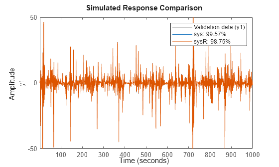
The large negative fit result for the unregularized model indicates a poor fit to the data. Estimating a regularized model produces a significantly better result.
Load the estimation data.
load twotankdata y u
Create an iddata object from the data. Use the first 1000 samples for estimation and the remaining samples for validation.
Ts = 0.2;
z = iddata(y,u,Ts);
ze = z(1:1000);
zv = z(1001:end);
Create an nlarxOptions option set. Specify a simulation error minimization objective, 'lm' least squares search, and a maximum of 10 estimation iterations. Display progress during estimation.
opt = nlarxOptions('Focus','simulation','SearchMethod','lm','Display','on');
opt.SearchOptions.MaxIterations = 10;
Estimate a nonlinear ARX model, using ARX model orders to specify the regressors and an idSigmoidNetwork mapping function. The model uses all candidate regressors. To view regressor usage information, at the MATLAB® command prompt, enter sys.RegressorUsage.
orders = [8 8 1];
outputFcn = idSigmoidNetwork;
sys = nlarx(ze,orders,outputFcn,opt);
allRegressors = getreg(sys);
rng default
Sparsify the model (reduce the regressors in use) by using the "log-sum" measure.
opt.SearchOptions.MaxIterations = 20;
opt.SparsifyRegressors = true;
opt.SparsificationOptions.MaxIterations = 10;
opt.SparsificationOptions.Lambda = 0.75;
sysr1 = nlarx(ze,sys,opt);
T = sysr1.RegressorUsage;
inUse = any(T{:,:},2);
fprintf('Regressors in use: %s\n', strjoin(allRegressors(inUse),', '))
Regressors in use: u1(t-4), u1(t-8)
Sparsify the model again using the "l1" measure.
opt.SparsificationOptions.SparsityMeasure = 'l1';
opt.SparsificationOptions.Lambda = 2.2;
sysr2 = nlarx(ze,sys,opt);
T = sysr2.RegressorUsage;
inUse = any(T{:,:},2);
fprintf('Regressors in use: %s\n', strjoin(allRegressors(inUse),', '))
Regressors in use: y1(t-1), y1(t-2), y1(t-3), y1(t-4), y1(t-5), y1(t-6), y1(t-7), y1(t-8), u1(t-8)
Sparsify the model again using the "l0" measure.
opt.SparsificationOptions.SparsityMeasure = 'l0';
opt.SparsificationOptions.Lambda = 2.2;
sysr3 = nlarx(ze,sys,opt);
T = sysr3.RegressorUsage;
InUse = any(T{:,:},2);
fprintf('Regressors in use: %s\n', strjoin(allRegressors(inUse),', '))
Regressors in use: y1(t-1), y1(t-2), y1(t-3), y1(t-4), y1(t-5), y1(t-6), y1(t-7), y1(t-8), u1(t-8)
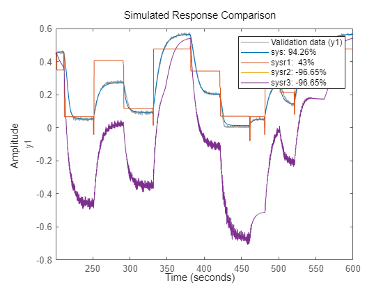
Compare the full regressor model and three sparse regressor models against the validation data.
compare(zv,sys,sysr1,sysr2,sysr3)
Input Arguments
Name-Value Arguments
Output Arguments
Algorithms
A nonlinear ARX model consists of model regressors and an output function. The output function contains one or more mapping objects, one for each model output. Each mapping object can include a linear and a nonlinear function that act on the model regressors to give the model output and a fixed offset for that output. This block diagram represents the structure of a single-output nonlinear ARX model in a simulation scenario.
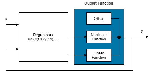
The software computes the nonlinear ARX model output y in two stages:
It computes regressor values from the current and past input values and the past output data.
In the simplest case, regressors are delayed inputs and outputs, such as u(t–1) and y(t–3). These kind of regressors are called linear regressors. You specify linear regressors using the
linearRegressorobject. You can also specify linear regressors by using linear ARX model orders as an input argument. For more information, see Nonlinear ARX Model Orders and Delay. However, this second approach constrains your regressor set to linear regressors with consecutive delays. To create polynomial regressors, use thepolynomialRegressorobject. To create periodic regressors that contain the sine and cosine functions of delayed input and output variables, use theperiodicRegressorobject. You can also specify custom regressors, which are nonlinear functions of delayed inputs and outputs. For example, u(t–1)y(t–3) is a custom regressor that multiplies instances of input and output together. Specify custom regressors using thecustomRegressorobject.You can assign any of the regressors as inputs to the linear function block of the output function, the nonlinear function block, or both.
It maps the regressors to the model output using an output function block. The output function block can include multiple mapping objects, with each mapping object containing linear, nonlinear, and offset blocks in parallel. For example, consider the following equation:
Here, x is a vector of the regressors, and r is the mean of x. is the output of the linear function block. represents the output of the nonlinear function block. Q is a projection matrix that makes the calculations well-conditioned. d is a scalar offset that is added to the combined outputs of the linear and nonlinear blocks. The exact form of F(x) depends on your choice of output function. You can select from the available mapping objects, such as tree-partition networks, wavelet networks, and multilayer neural networks. You can also exclude either the linear or the nonlinear function block from the output function.
When estimating a nonlinear ARX model, the software computes the model parameter values, such as L, r, d, Q, and other parameters specifying g.
The resulting nonlinear ARX models are idnlarx objects that store all model data, including model regressors and
parameters of the output function. For more information about these objects, see Nonlinear Model Structures.
Version History
Introduced in R2007aSee Also
idnlarx | nlarxOptions | isnlarx | goodnessOfFit | aic | fpe | polynomialRegressor | periodicRegressor | linearRegressor | customRegressor
Topics
- Estimate Nonlinear ARX Models at the Command Line
- Estimate Nonlinear ARX Models Initialized Using Linear ARX Models
- Identifying Nonlinear ARX Models
- Validate Nonlinear ARX Models
- Using Nonlinear ARX Models
- Loss Function and Model Quality Metrics
- Regularized Estimates of Model Parameters
- Estimation Report
- Cascade-Correlation Neural Networks