Identifying Nonlinear ARX Models
Nonlinear ARX models extend the linear ARX model to the nonlinear case. For information about the structure of nonlinear ARX models, see What Are Nonlinear ARX Models?
You can estimate nonlinear ARX models in the System Identification app or at
the command line using the nlarx command.
To estimate a nonlinear ARX model, you first prepare the estimation
data. You then configure the model structure and estimation algorithm,
and then perform the estimation. After estimation, you can validate
the estimated model as described in Validate Nonlinear ARX Models.
Prepare Data for Identification
You can use uniformly sampled time-domain input-output data or time-series data (no inputs) for estimating nonlinear ARX models. Your data can have zero or more input channels and one or more output channels. You cannot use frequency-domain data for estimation.
To prepare the data for model estimation, import your data into the MATLAB® workspace, and do one of the following:
In the System Identification app — Import data into the app, as described in Represent Data.
At the command line — Represent your data as an
iddataobject.
After importing the data, you can analyze data quality and preprocess data by interpolating missing values, filtering to emphasize a specific frequency range, or resampling using a different sample time. For more information, see Data Preparation. For most applications, you do not need to remove offsets and linear trends from the data before nonlinear modeling. However, data detrending can be useful in some cases, such as before modeling the relationship between the change in input and output about an operating point.
After preparing your estimation data, you can configure your model structure, loss function, and estimation algorithm, and then estimate the model using the estimation data.
Configure Nonlinear ARX Model Structure
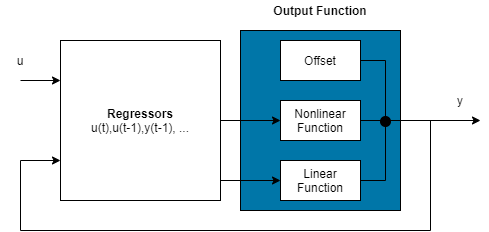
A nonlinear ARX model consists of a set of regressors that can be any combination of linear, polynomial, and custom regressors, and an output function that typically contains a nonlinear and a linear component, as well as a static offset. The block diagram represents the structure of a nonlinear ARX model in a simulation scenario.
To configure the structure of a nonlinear ARX model:
Configure the model regressors.
Choose the linear, polynomial, and customer regressors based on your knowledge of the physical system you are trying to model.
Specify linear regressors in one of the following ways:
Specify model orders and delay to create the set of linear regressors. For more information, see Nonlinear ARX Model Orders and Delay.
Directly specify the linear regressors by constructing and using
linearRegressorobjects.Initialize the model using a linear ARX model. You can perform this operation at the command line only. The initialization configures the nonlinear ARX model to use the linear regressors of the linear model. For more information, see Initialize Nonlinear ARX Estimation Using Linear Model.
Specify polynomial regressors and custom regressors. Polynomial regressors are polynomials that are composed of delayed input and output variables. Custom regressors are arbitrary functions of past inputs and outputs, such as products, powers, and other MATLAB expressions of input and output variables. Specify polynomial and custom regressors in addition to, or instead of, linear regressors for greater flexibility in modeling your data. For more information, see
polynomialRegressorandcustomRegressor.Assign regressors as inputs to the linear and nonlinear components of the output function block. Any regressor can be assigned to either or both of these components. Limiting the number of regressors that are input to the nonlinear component can help reduce model complexity and keep the estimation well conditioned.
The choice of regressors to use for each component can require multiple trials. You can examine a nonlinear ARX plot to help you gain insight into which regressors have the strongest effect on the model output. Understanding the relative importance of the regressors on the output can then help you decide how to assign the regressors.
Configure the output function block.
Specify and configure the output function F(x).
Here, x is a vector of the regressors, and r is the mean of the regressors x. is the output of the linear function block. represents the output of the nonlinear function block. Q is a projection matrix that makes the calculations well conditioned. d is a scalar offset that is added to the combined outputs of the linear and nonlinear blocks. The exact form of F(x) depends on your choice of output function. You can select from available nonlinearity estimators, such as tree-partition networks, wavelet networks, and multilayer neural networks. You can also exclude either the linear or the nonlinear function block from the output function.
You can also perform one of the following tasks:
Exclude the nonlinear function from the output function such that F(x) = .
Exclude the linear function from the output function such that F(x) = .
Note
You cannot exclude the linear function from tree partitions and neural networks.
For information about how to configure the model structure at the command line and in the app, see Estimate Nonlinear ARX Models at the Command Line and Estimate Nonlinear ARX Models in the App.
Specify Estimation Options for Nonlinear ARX Models
To configure the model estimation, specify the loss function to be minimized, and choose the estimation algorithm and other estimation options to perform the minimization.
Configure Loss Function
The loss function or cost function is a function of the error between the model output and the measured output. For more information about loss functions, see Loss Function and Model Quality Metrics.
At the command line, use the nlarx option
set, nlarxOptions to configure
your loss function. You can specify the following options:
Focus— Specifies whether the simulation or prediction error is minimized during parameter estimation. By default, the software minimizes one-step prediction errors, which correspond to aFocusvalue of'prediction'. If you want a model that is optimized for reproducing simulation behavior, specifyFocusas'simulation'. Minimization of simulation error requires differentiable nonlinear functions and takes more time than one-step-ahead prediction error minimization. Thus, you cannot useidTreePartitionandidNeuralNetworknonlinearities when minimizing the simulation error because these nonlinearity estimators are not differentiable.OutputWeight— Specifies a weighting of the error in multi-output estimations.Regularization— Modifies the loss function to add a penalty on the variance of the estimated parameters. For more information, see Regularized Estimates of Model Parameters.
Specify Estimation Algorithm
To estimate a nonlinear ARX model, the software uses iterative
search algorithms to minimize the error between the simulated or predicted
model output and the measured output. At the command line, use nlarxOptions to
specify the search algorithm and other estimation options. Some of
the options you can specify are:
SearchMethod— Search method for minimization of prediction or simulation errors, such as Gauss-Newton and Levenberg-Marquardt line search, and Trust-Region-Reflective Newton approach.SearchOptions— Option set for the search algorithm, with fields that depend on the value ofSearchMethod, such as:MaxIterations— Maximum number of iterations.Tolerance— Condition for terminating iterative search when the expected improvement of the parameter values is less than a specified value.
To see a complete list of available estimation options, see nlarxOptions. For details about how to
specify these estimation options in the app, see Estimate Nonlinear ARX Models in the App.
After preprocessing the estimation data and configuring the
model structure and estimation options, you can estimate the model
in the System Identification app,
or using nlarx at the command
line. The resulting model is an idnlarx object
that stores all model data, including model regressors and parameters
of the nonlinearity estimator. For more information about these model
objects, see Nonlinear Model Structures. You can validate the estimated
model as described in Validate Nonlinear ARX Models.
Initialize Nonlinear ARX Estimation Using Linear Model
At the command line, you can use an ARX structure polynomial
model (idpoly with only A and B as
active polynomials) for nonlinear ARX estimation. To learn more about
when to use linear models, see When to Fit Nonlinear Models.
Typically, you create a linear ARX model using the arx command. You can provide the linear
model when constructing or estimating a nonlinear ARX model. For example,
use the following syntax to estimate a nonlinear ARX model using estimation
data and a linear ARX model LinARXModel.
m = nlarx(data,LinARXModel)
Here m is an idnlarx object,
and data is a time-domain iddata object.
The software uses the linear model for initializing the nonlinear
ARX estimation by:
Assigning the linear ARX model orders and delays as initial values of the nonlinear ARX model orders (
naandnbproperties of theidnlarxobject) and delays (nkproperty). The software uses these orders and delays to compute linear regressors in the nonlinear ARX model structure.Using the A and B polynomials of the linear model to compute the linear function of the nonlinearity estimators (
LinearCoefparameter of the nonlinearity estimator object), except if the nonlinearity estimator is a neural network.
During estimation, the estimation algorithm uses these values to adjust the nonlinear model to the data.
Note
When you use the same data for estimation, a nonlinear ARX model initialized using a linear ARX model produces a better fit to measured output than the linear ARX model itself.
By default, the nonlinearity estimator is the wavelet network (idWaveletNetwork object). You can also
specify different input and output nonlinearity estimators. For example, you can
specify a sigmoid network nonlinearity estimator.
m = nlarx(data,LinARXModel,'idSigmoidNetwork')For an example, see Estimate Nonlinear ARX Models Initialized Using Linear ARX Models.