cwtLayer
Description
A CWT layer computes the continuous wavelet transform of the input. Use of this layer requires Deep Learning Toolbox™.
Creation
Description
layer = cwtLayer
The input to cwtLayer must be a real-valued dlarray (Deep Learning Toolbox) object in
"CBT" format. The size along the time dimension of the tensor input
is padded to equal the value of SignalLength. By default, cwtLayer formats the output as
"SCBT". For more information, see Layer Output Format.
Note
When you initialize the learnable parameters of cwtLayer, the
layer weights are set to the wavelet filters used in the CWT. It is not recommended to
initialize the weights directly.
layer = cwtLayer(PropertyName=Value)layer = cwtLayer(SignalLength=2048,VoicesPerOctave=14) creates
a layer for a signal of length 2048 in the time dimension that uses 14 voices per octave
in the CWT. You can specify multiple name-value arguments.
Note
You cannot use this syntax to set the Weights
property.
Example: cwtl = cwtLayer(Wavelet="amor",VoicesPerOctave=24)
creates a CWT layer with a Morlet (Gabor) wavelet and 24 voices per octave.
Properties
CWT
This property is read-only after object creation.
Signal length in samples, specified as a positive integer greater than or equal
to 4. All sequence inputs to cwtLayer are padded to have size
SignalLength along the time dimension.
You can set this property when you create the cwtLayer object. After you create the object, this property is read-only.
Data Types: single | double
This property is read-only after object creation.
Analysis wavelet used in the CWT, specified as "Morse",
"amor", or "bump", representing the analytic
Morse, Morlet (Gabor), and bump wavelet, respectively. The default wavelet is the
analytic Morse (3,60) wavelet.
You can set this property when you create the cwtLayer object. After you create the object, this property is read-only.
This property is read-only after object creation.
Weight threshold, specified as a positive real scalar. cwtLayer
uses the threshold value to determine the significant values for each of the CWT
filters in the wavelet filter bank prior to any weight modification through learning.
It sets values below the specified threshold to zero and excludes them from learning.
The CWT filters are normalized so that the peak value is 2 for each filter.
Smaller values of
Thresholdresult in more values being retained from the CWT filters and therefore less weight reduction.Larger values of
Thresholdresult in more weight reduction and more divergence between the deep learning CWT and transforms computed with the full filter bank.A threshold less than
realmin, the smallest positive normalized floating-point number in double precision, is clipped torealminfor computing significant filter values.
Setting Threshold to a value which results in no
values being retained for any individual filter results in an error.
You can set this property when you create the cwtLayer object. After you create the object, this property is read-only.
Data Types: single | double
This property is read-only after object creation.
Include lowpass filter, specified as a numeric or logical 1
(true) or 0 (false).
Specify true to include the lowpass (scaling) filter in the
CWT.
You can set this property when you create the cwtLayer object. After you create the object, this property is read-only.
Data Types: logical
This property is read-only after object creation.
Number of voices per octave in the CWT, specified as an integer between 1 and 48. The CWT scales are discretized using the specified number of voices per octave. The energy spread of the wavelet in frequency and time automatically determines the minimum and maximum scales.
You can use cwtfreqbounds to determine the frequency limits of the wavelet filter
bank. The frequency limits depend on parameters such as the energy spread of the
wavelet, number of voices per octave, and signal length.
You can set this property when you create the cwtLayer object. After you create the object, this property is read-only.
Data Types: single | double
This property is read-only after object creation.
Frequency limits for the CWT, specified as a two-element vector with positive strictly increasing entries. The frequency limits are interpreted as normalized frequencies, cycles/sample.
The first element specifies the lowest peak passband frequency and must be greater than or equal to the product of the wavelet peak frequency in normalized frequency and two time standard deviations divided by SignalLength.
The second element specifies the highest peak passband frequency and must be less than or equal to the Nyquist frequency.
The base-2 logarithm of the ratio of the upper frequency limit
freqMax to the lower frequency limit freqMin
must be greater than or equal to 1/VoicesPerOctave:
log2(freqMax/freqMin) ≥
                    1/VoicesPerOctave
.
For more information, see CWT Frequency Limits.
To obtain normalized frequencies, divide your desired frequency limits in hertz by the sample rate in hertz. For example, if the sample rate is 1000 Hz and your desired frequency limits are [100,400] Hz, divide each element by 1000 to obtain the normalized frequencies: [100/1000,400/1000].
Frequency limits apply only to wavelet filters. If you additionally specify
IncludeLowpass as true,
cwtLayer also includes the lowpass (scaling) filter.
You can set this property when you create the cwtLayer object. After you create the object, this property is read-only.
Note
If you use Deep Network
Designer (Deep Learning Toolbox) to create or edit a deep learning network, and change the
Wavelet property of a cwtLayer, the app does not change the frequency limits of the layer.
If you want the app to provide the default frequency limits appropriate for the new
wavelet, you must take additional steps. For more information, see Reset Frequency Limits to Default Values in Deep Network Designer.
Data Types: single | double
This property is read-only after object creation.
Time-bandwidth product for the Morse wavelet, specified as a positive scalar
greater than or equal to 3 and less than or equal to 120. The symmetry (gamma) of the
Morse wavelet is fixed at 3. This property is only valid when
Wavelet is "Morse". The layer ignores the
time-bandwidth product for the "amor" and "bump"
wavelets. For Morse wavelets, the larger the time-bandwidth product, the more spread
out the wavelet is in time and narrower the wavelet is in frequency.
In the notation of Morse Wavelets,
TimeBandwidth is
P2.
You can set this property when you create the cwtLayer object. After you create the object, this property is read-only.
Data Types: single | double
Layer transform mode, specified as one of these:
"mag"— CWT magnitude"squaremag"— CWT squared magnitude"realimag"— CWT real and imaginary parts concatenated along the channel dimension
Layer
Layer weights, specified as [], a numeric
array, or a dlarray object.
The layer weights are learnable parameters.
You can use initialize (Deep Learning Toolbox)
to initialize the learnable parameters of a dlnetwork (Deep Learning Toolbox) that includes
cwtLayer objects. When you initialize the layers,
initialize sets Weights to the CWT filter
bank associated with the specified Wavelet. For more information,
see Initialize Continuous Wavelet Transform Layer (since R2025a)
It is not recommended to initialize the weights directly.
Data Types: single | double
Multiplier for weight learning rate, specified as a nonnegative scalar. The
weights are the reduced CWT filter values represented as a
1-by-1-by-Nr tensor. See cwtfilters2array for details. By default, the weights do not update with
training.
Data Types: single | double
This property is read-only.
Number of inputs to the layer, stored as 1. This layer accepts a
single input only.
Data Types: double
This property is read-only.
Input names, stored as {'in'}. This layer accepts a single input
only.
Data Types: cell
This property is read-only.
Number of outputs from the layer, stored as 1. This layer has a
single output only.
Data Types: double
This property is read-only.
Output names, stored as {'out'}. This layer has a single output
only.
Data Types: cell
Object Functions
filterbank | Full-weight CWT filter bank for deep learning |
Examples
Create a CWT layer for a signal of length 2000 samples. Set the learning rate factor to 1.
cLayer = cwtLayer(SignalLength=2000,WeightLearnRateFactor=1);
Create a three-layer dlnetwork containing a sequence input layer, the CWT layer you just made, and a 2-D max pooling layer.
sqLayer = sequenceInputLayer(1,Name="input",MinLength=2000);
mpLayer = maxPooling2dLayer([2 25],Stride=[2 12]);
layers = [sqLayer
    cLayer
    mpLayer];
dlnet = dlnetwork(layers);
Run a batch of 10 random single-channel signals through the dlnetwork.
dataout = forward(dlnet, ...
    dlarray(randn(1,10,2000,"single"),"CBT"));
size(dataout)
ans = 1×4

    40     1    10   165
dims(dataout)
ans =
'SCBT'
Load the Espiga3 EEG dataset. The data consists of 23 channels of EEG sampled at 200 Hz. There are 995 samples in each channel. Save the multisignal as a dlarray, specifying the dimensions in order. dlarray permutes the array dimensions to the "CBT" shape expected by a deep learning network.
load Espiga3
[N,nch] = size(Espiga3);
x = dlarray(Espiga3,"TCB");
whos Espiga3 x
  Name           Size                Bytes  Class      Attributes

  Espiga3      995x23               183080  double
  x             23x1x995            183110  dlarray
Create a CWT filter bank that is appropriate for the channels in the dataset. Use the default analytic Morse (3,60) wavelet. Specify periodic boundary conditions. Use the filter bank to obtain the CWT of one of the channels. The CWT is a 2-D matrix. The row dimension corresponds to scale, or frequency, and the column dimension corresponds to time.
fb = cwtfilterbank(SignalLength=N,Boundary="periodic");
colInd = 11;
cfs = wt(fb,Espiga3(:,colInd));
Layer Transform Mode — "mag"
Create a CWT layer that can be used with the EEG data. By default, the layer outputs the absolute value of the CWT, or scalogram, of each channel.
clayer = cwtLayer(SignalLength=N);
Create a two-layer dlnetwork object containing a sequence input layer and the CWT layer you just created. Treat each channel as a feature. Specify the signal length as the minimum sequence length for the input layer.
slayer = sequenceInputLayer(nch,MinLength=N);
layers = [slayer
    clayer];
dlnet = dlnetwork(layers);
Run the EEG data through the forward method of the network.
dataout = forward(dlnet,x);
By default, the output of cwtLayer is a dlarray object in "SCBT" format. The spatial dimension corresponds to frequency. Convert the network output to a numeric array. Permute the dimensions of the network output to correspond with "STCB" format. The result is a 3-D numeric array because there is only one batch.
q = extractdata(dataout);
q = permute(q,[1 4 2 3]);
whos q cfs
  Name       Size                  Bytes  Class     Attributes

  cfs       71x995               1130320  double    complex
  q         71x995x23            6499340  single
Extract from the output the result that corresponds to the channel you chose. Compare with the absolute value of the CWT you obtained previously.
r = q(:,:,colInd);
d = max(abs(r(:)-abs(cfs(:))));
str = sprintf("Difference: %g",d);
fprintf("%s\n",str)
Difference: 8.86966e-06
subplot(2,1,1)
imagesc(r)
title("Layer Output")
subplot(2,1,2)
imagesc(abs(cfs))
title("Filter Bank Output")

Layer Transform Mode — "realimag"
Create a CWT layer that can be used with the data. Specify the layer outputs to be the real and imaginary parts of the CWT. Create a two-layer dlnetwork object containing a sequence input layer and the CWT layer. Run the EEG data through the forward method of the network.
clayer2 = cwtLayer(SignalLength=N,TransformMode="realimag");
layers2 = [slayer
    clayer2];
dlnet2 = dlnetwork(layers2);
dataout2 = forward(dlnet2,x);
Convert the network output to a numeric array. Permute the dimensions of the network output to correspond with "STCB" format. Because the output are the real and imaginary parts of the CWT, the size of the channel dimension is twice the number of input channels.
q2 = extractdata(dataout2);
q2 = permute(q2,[1 4 2 3]);
whos q2
Name Size Bytes Class Attributes q2 71x995x46 12998680 single
Choose a channel. Use the CWT filter bank to obtain the CWT of that channel. Compare the real and imaginary parts of the CWT with the corresponding results from the network output.
colInd = 23;
cfs = wt(fb,Espiga3(:,colInd));
r = q2(:,:,[colInd nch+colInd]);

a1 = real(cfs);
a2 = r(:,:,1);
str1 = sprintf("Difference (real part): %g",max(abs(a1(:)-a2(:))));

a1 = imag(cfs);
a2 = r(:,:,2);
str2 = sprintf("Difference (imag part): %g",max(abs(a1(:)-a2(:))));

fprintf("%s\n%s\n",str1,str2)
Difference (real part): 7.102e-05
Difference (imag part): 6.94453e-05
figure
subplot(2,2,1)
imagesc(real(cfs))
title("Filter Bank — Real")
subplot(2,2,2)
imagesc(r(:,:,1))
title("Layer — Real")
subplot(2,2,3)
imagesc(imag(cfs))
title("Filter Bank — Imag")
subplot(2,2,4)
imagesc(r(:,:,2))
title("Layer — Imag")

Create a CWT layer using default values. By default, the CWT layer is for a signal length of 1024 samples. The layer uses the analytic Morse (3,60) wavelet in the CWT with 10 voices per octave and periodic boundary conditions. Inspect the default frequency limits of the layer. The frequency limits, which are in units of cycles/sample, are based on the energy spread of the wavelet, the signal length, and the voices per octave.
clayer = cwtLayer;
clayer.FrequencyLimits
ans = 1×2

    0.0032    0.4341
Use the filterbank method of the layer to obtain the full-weight CWT filter bank for the layer. Each row contains the values of a filter. The filters are ordered from high center frequency to low.
psif = filterbank(clayer);
whos psif
Name Size Bytes Class Attributes psif 71x1024 290816 single
You can determine the center frequencies by creating a cwtfilterbank object, specifying the same wavelet parameters as used in the CWT layer, and then use the centerFrequencies object function.
Create a cwtfilterbank. The default wavelet parameters are identical to those in the CWT layer. Obtain the center frequencies. The frequencies are ordered from high to low. Plot the center frequencies.
fb = cwtfilterbank;
cf = centerFrequencies(fb);
subplot(2,1,1)
plot(cf)
ylabel("Cycles/Sample")
title("Wavelet Center Frequencies")
grid on
subplot(2,1,2)
semilogy(cf)
grid on
ylabel("Cycles/Sample")
title("Semi-Log Scale")

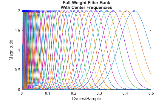
The plots show that the wavelet center frequencies are not linearly spaced as is commonly the case with other filter banks. Specifically, the center frequencies are exponentially decreasing. In continuous wavelet analysis, the center frequencies of the wavelet filters are logarithmically spaced. The most common spacing is the base 2^(1/NV), where NV is the number of voices per octave, raised to integer powers. In other words, in a CWT filter bank, it is not possible for consecutive center frequencies and , where , to satisfy . Frequency limits you specify in the CWT layer must satisfy .
The CWT layer uses 10 voices per octave. Compute the base-2 logarithm of the ratios of consecutive pairs of center frequencies. Confirm the minimum and maximum values of the result are both equal to 1/10.
cfRatio = log2(cf(1:end-1)./cf(2:end));
[min(cfRatio) max(cfRatio)]
ans = 1×2

    0.1000    0.1000
Plot the full-weight CWT filter bank and the center frequencies. The center frequencies correspond to the peaks of the frequency response of each wavelet in the filter bank.
slen = clayer.SignalLength;
f = 0:1/slen:1-1/slen;
figure
plot(f,psif')
xlim([0 1/2])
xlabel("Cycles/Sample")
ylabel("Magnitude")
title(["Full-Weight Filter Bank", "With Center Frequencies"])
hold on
plot(cf,2*ones(size(psif,1),1),'bx')
hold off
If the CWT layer you created does not support your frequency limits, try increasing the number of voices per octave in the layer. For more information, see Practical Introduction to Time-Frequency Analysis Using the Continuous Wavelet Transform and Continuous and Discrete Wavelet Transforms.
Reset the frequency limits to default values after changing the wavelet of a cwtLayer in Deep Network Designer.
Suppose you are editing a deep learning network using Deep Network Designer. The network has a cwtLayer that uses the Morse wavelet and has frequency limits set at [0.1,0.3].
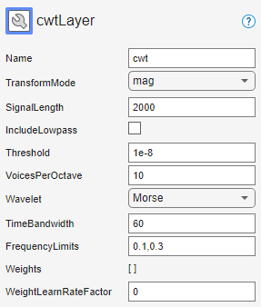
Use the drop-down list to change the Wavelet to amor. The frequency limits do not change.
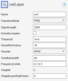
To change the frequency limits to default values appropriate for the amor wavelet, first do one of the following:
Delete the FrequencyLimits
0.1,0.3.Set the FrequencyLimits to
[].
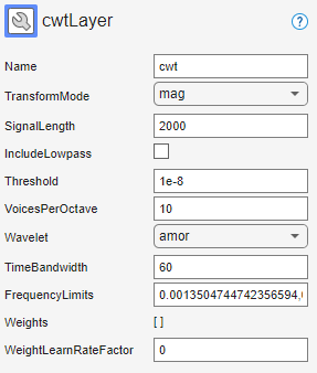
Then click the mouse outside the FrequencyLimits edit field to move the focus. The app automatically populates FrequencyLimits with default values for the amor wavelet.
Tip: If you change the frequency limits, and later want to restore the default values, follow the same steps.
Since R2025a
Verify that the weights of a continuous wavelet transform (CWT) layer are reset to the specified wavelet when you reinitialize the containing network.
Define an array of seven layers: a sequence input layer, a CWT layer, a 2-D convolutional layer, a batch normalization layer, a rectified linear unit (ReLU) layer, a fully connected layer, and a softmax layer. There is one feature in the sequence input. Set the minimum signal length in the sequence input layer to 250 samples. Use a signal length of 256 samples and a bump wavelet for the CWT layer.
sL = 256;
wName = "bump";
layers = [
   sequenceInputLayer(1,MinLength=250)
   cwtLayer(SignalLength=sL,Wavelet=wName,Name="cwt")
   convolution2dLayer(4,15,Padding="same")
   batchNormalizationLayer
   reluLayer
   fullyConnectedLayer(3)
   softmaxLayer];
Create a deep learning neural network from the layer array. By default, the dlnetwork function initializes the network at creation. For reproducibility, use the default random number generator.
rng("default")
net = dlnetwork(layers);
Display the table of learnable parameters. The network weights and bias are nonempty dlarray objects.
tInit1 = net.Learnables
tInit1=7×3 table
       Layer       Parameter          Value
    ___________    _________    __________________

    "cwt"          "Weights"    {1×1×375  dlarray}
    "conv"         "Weights"    {4×4×1×15 dlarray}
    "conv"         "Bias"       {1×1×15   dlarray}
    "batchnorm"    "Offset"     {1×15     dlarray}
    "batchnorm"    "Scale"      {1×15     dlarray}
    "fc"           "Weights"    {3×555    dlarray}
    "fc"           "Bias"       {3×1      dlarray}
Extract the filter bank from the CWT layer.
psif1 = filterbank(net.Layers(2));
Compare the initialized weights of the CWT layer from the list of learnable parameters with the reduced-weight CWT filter tensor of the corresponding CWT filter bank. The cwtLayer weights are single precision and initialized to the specified wavelet.
fb = cwtfilterbank(SignalLength=sL,Wavelet=wName,Boundary="periodic");
psifvec = cwtfilters2array(fb);
psifLayer = tInit1.Value{1};
isequal(single(psifvec),psifLayer)
ans = logical
1
Set the learnable parameters to empty arrays.
net = dlupdate(@(x)[],net);
net.Learnables
ans=7×3 table
       Layer       Parameter       Value
    ___________    _________    ____________

    "cwt"          "Weights"    {0×0 double}
    "conv"         "Weights"    {0×0 double}
    "conv"         "Bias"       {0×0 double}
    "batchnorm"    "Offset"     {0×0 double}
    "batchnorm"    "Scale"      {0×0 double}
    "fc"           "Weights"    {0×0 double}
    "fc"           "Bias"       {0×0 double}
Reinitialize the network and extract the filter bank from the CWT layer. Display the network and the learnable parameters. The network weights and bias are nonempty dlarray objects.
net = initialize(net);
psif2 = filterbank(net.Layers(2));
tInit2 = net.Learnables
tInit2=7×3 table
       Layer       Parameter          Value
    ___________    _________    __________________

    "cwt"          "Weights"    {1×1×375  dlarray}
    "conv"         "Weights"    {4×4×1×15 dlarray}
    "conv"         "Bias"       {1×1×15   dlarray}
    "batchnorm"    "Offset"     {1×15     dlarray}
    "batchnorm"    "Scale"      {1×15     dlarray}
    "fc"           "Weights"    {3×555    dlarray}
    "fc"           "Bias"       {3×1      dlarray}
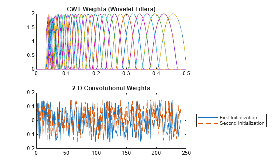
Compare the weights from the CWT and 2-D convolutional layers along the two initialization calls. The CWT layer sets the weights using the specified wavelet, while the convolutional layer weights consists of a new set of random values.
tiledlayout flow
ff = 0:1/sL:1-1/sL;
nexttile
plot(ff,psif1')
xlim([0 1/2])
hold on
plot(ff,psif2',"--")
hold off
title("CWT Weights (Wavelet Filters)")
nexttile
plot(tInit1.Value{2}(:))
hold on
plot(tInit2.Value{2}(:),"--")
hold off
title("2-D Convolutional Weights")
legend(["First" "Second"] + " Initialization", ...
    Location="eastoutside")
More About
cwtLayer formats the output as
"SCBT", a sequence of 1-D images where the image height corresponds to
scale, or frequency. The second dimension corresponds to the channel, the third dimension
corresponds to the batch, and the fourth dimension corresponds to time.
You can feed the output of
cwtLayerunchanged to a 1-D convolutional layer when you want to convolve along the frequency ("S") dimension. For more information, seeconvolution1dLayer(Deep Learning Toolbox).To feed the output of
cwtLayerto a 1-D convolutional layer when you want to convolve along the time ("T") dimension, you must place a flatten layer after thecwtLayer. For more information, seeflattenLayer(Deep Learning Toolbox).You can feed the output of
cwtLayerunchanged to a 2-D convolutional layer when you want to convolve along the frequency ("S") and time ("T") dimensions jointly. For more information, seeconvolution2dLayer(Deep Learning Toolbox).To use
cwtLayeras part of a recurrent neural network, you must place a flatten layer after thecwtLayer. For more information, seelstmLayer(Deep Learning Toolbox) andgruLayer(Deep Learning Toolbox).To use the output of
cwtLayerwith a fully connected layer as part of a classification workflow, you must reduce the time ("T") dimension of the output so that it has size 1. To reduce the time dimension of the output, place a global pooling layer before the fully connected layer. For more information, seeglobalAveragePooling2dLayer(Deep Learning Toolbox) andfullyConnectedLayer(Deep Learning Toolbox).
Tips
For the best reconstruction when the filters in
cwtLayerandicwtLayerare not learnable (which is the default setting):Ensure consistency in the filter bank used for the CWT and ICWT by using the same parameters in
cwtLayerandicwtLayer.Include the scaling coefficients by setting
IncludeLowpasstotrueincwtLayerandicwtLayer.
Extended Capabilities
C/C++ Code Generation
Generate C and C++ code using MATLAB® Coder™. (since R2026a)
GPU Code Generation
Generate CUDA® code for NVIDIA® GPUs using GPU Coder™. (since R2026a)
Version History
Introduced in R2022bThe cwtLayer object supports:
C/C++ code generation. You must have MATLAB® Coder™ to generate C/C++ code.
Code generation for NVIDIA® GPUs. You must have GPU Coder™ to generate GPU code.
Starting in R2025a, you can use initialize (Deep Learning Toolbox) to
initialize learnable parameters for deep learning neural networks that include
cwtLayer objects.
Starting in R2025a, the default value of the Weights property is
[]. Prior to R2025a, cwtLayer set the default value
to the wavelet filters used in the CWT.
See Also
Apps
- Deep Network Designer (Deep Learning Toolbox)
Functions
dlcwt|dlicwt|cwt|icwt|cwtfreqbounds|cwtfilters2array|array2cwtfilters
Objects
icwtLayer|cwtfilterbank|dlarray(Deep Learning Toolbox) |dlnetwork(Deep Learning Toolbox)
Topics
- Practical Introduction to Time-Frequency Analysis Using the Continuous Wavelet Transform
- Time-Frequency Convolutional Network for EEG Data Classification
- Time-Frequency Feature Embedding with Deep Metric Learning
- Deep Learning in MATLAB (Deep Learning Toolbox)
- List of Deep Learning Layers (Deep Learning Toolbox)
- Networks and Layers Supported for Code Generation (MATLAB Coder)
- Supported Networks, Layers, and Classes (GPU Coder)
MATLAB Command
You clicked a link that corresponds to this MATLAB command:
Run the command by entering it in the MATLAB Command Window. Web browsers do not support MATLAB commands.
Select a Web Site
Choose a web site to get translated content where available and see local events and offers. Based on your location, we recommend that you select: .
You can also select a web site from the following list
How to Get Best Site Performance
Select the China site (in Chinese or English) for best site performance. Other MathWorks country sites are not optimized for visits from your location.
Americas
- América Latina (Español)
- Canada (English)
- United States (English)
Europe
- Belgium (English)
- Denmark (English)
- Deutschland (Deutsch)
- España (Español)
- Finland (English)
- France (Français)
- Ireland (English)
- Italia (Italiano)
- Luxembourg (English)
- Netherlands (English)
- Norway (English)
- Österreich (Deutsch)
- Portugal (English)
- Sweden (English)
- Switzerland
- United Kingdom (English)