Time-Frequency Feature Embedding with Deep Metric Learning
This example shows how to use deep metric learning with a supervised contrastive loss to construct feature embeddings based on a time-frequency analysis of electroencephalographic (EEG) signals. The learned time-frequency embeddings reduce the dimensionality of the time-series data by a factor of 16. You can use these embeddings to classify EEG time-series from persons with and without epilepsy using a support vector machine classifier.
Deep Metric Learning
Deep metric learning attempts to learn a nonlinear feature embedding, or encoder, that reduces the distance (a metric) between examples from the same class and increases the distance between examples from different classes. Loss functions that work in this way are often referred to as contrastive. This example uses supervised deep metric learning with a particular contrastive loss function called the normalized temperature-scaled cross-entropy loss [3],[4],[8]. The figure shows the general workflow for this supervised deep metric learning.
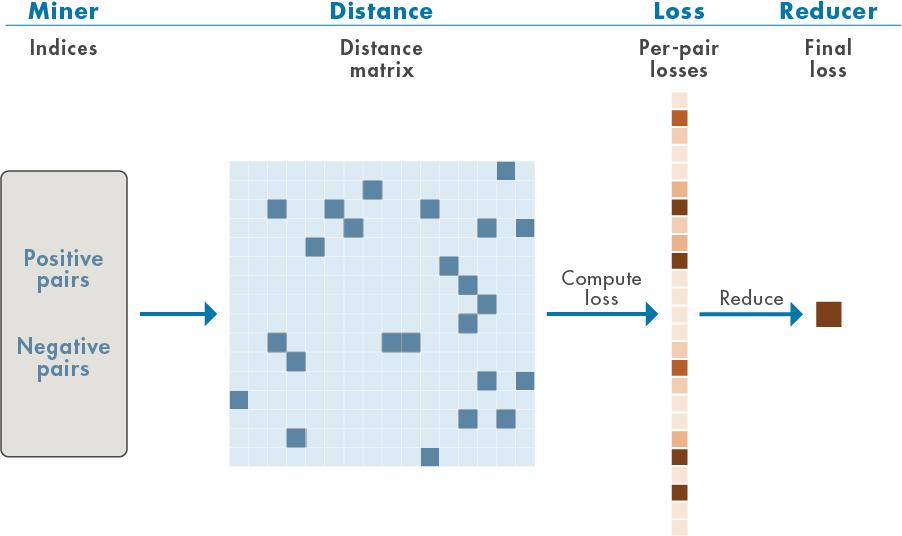
Positive pairs refer to training samples with the same label, while negative pairs refer to training samples with different labels. A distance, or similarity, matrix is formed from the positive and negative pairs. In this example, the cosine similarity matrix is used. From these distances, losses are computed and aggregated (reduced) to form a single scalar-valued loss for use in gradient-descent learning.
Deep metric learning is also applicable in weakly supervised, self-supervised, and unsupervised contexts. There is a wide variety of distance (metrics) measures, losses, reducers, and regularizers that are employed in deep metric learning.
Data — Description, Attribution, and Download Instructions
The data used in this example is the Bonn EEG Data Set. The data is currently available at EEG Data Download and Ralph Andrzejak's EEG data download page. See Ralph Andrzejak's EEG data for legal conditions on the use of the data. The authors have kindly permitted the use of the data in this example.
The data in this example were first analyzed and reported in:
The data consists of five sets of 100 single-channel EEG recordings. The resulting single-channel EEG recordings were selected from 128-channel EEG recordings after visually inspecting each channel for obvious artifacts and satisfying a weak stationarity criterion. See the linked paper for details.
The original paper designates these five sets as A-E. Each recording is 23.6 seconds in duration sampled at 173.61 Hz. Each time series contains 4097 samples. The conditions are as follows:
A -- Normal subjects with eyes open
B -- Normal subjects with eyes closed
C -- Seizure-free recordings from patients with epilepsy. Recording from hippocampus in the hemisphere opposite the epileptogenic zone
D -- Seizure-free recordings obtained from patients with epilepsy. Recordings from epileptogenic zone.
E - Recordings from patients with epilepsy showing seizure activity.
The zip files corresponding to this data are labeled as z.zip (A), o.zip (B), n.zip (C), f.zip (D), and s.zip (E).
The example assumes you have downloaded and unzipped the zip files into folders named Z, O, N, F, and S respectively. In MATLAB® you can do this by creating a parent folder and using that as the OUTPUTDIR variable in the unzip command. This example uses the folder designated by MATLAB as tempdir as the parent folder. If you choose to use a different folder, adjust the value of parentDir accordingly. The following code assumes that all the .zip files have been downloaded into parentDir. Unzip the files by folder into a subfolder called BonnEEG.
parentDir = tempdir;
cd(parentDir)
mkdir('BonnEEG')
dataDir = fullfile(parentDir,'BonnEEG');
unzip('z.zip',dataDir)
unzip('o.zip',dataDir)
unzip('n.zip',dataDir)
unzip('f.zip',dataDir)
unzip('s.zip',dataDir)
Creating In-Memory Data and Labels
The individual EEG time series are stored as .txt files in each of the Z, N, O, F, and S folders under dataDir. Use a tabularTextDatastore to read the data. Create a tabular text datastore and create a categorical array of signal labels based on the folder names.
tds = tabularTextDatastore(dataDir,'IncludeSubfolders',true,'FileExtensions','.txt');
The zip files were created on a macOS and accordingly there may be a MACOSX folder created with unzip that results in extra files. If those exist, remove them.
extraTXT = contains(tds.Files,'__MACOSX');
tds.Files(extraTXT) = [];
Create labels for the data based on the first letter of the text file name.
labels = filenames2labels(tds.Files,'ExtractBetween',[1 1]);Each read of the tabular text datastore creates a table containing the data. Create a cell array of all signals reshaped as row vectors so they conform with the deep learning networks used in the example.
ii = 1;
eegData = cell(numel(labels),1);
while hasdata(tds)
    tsTable = read(tds);
    ts = tsTable.Var1;
    eegData{ii} = reshape(ts,1,[]);
    ii = ii+1;
end
Time-Frequency Feature Embedding Deep Network
Here we construct a deep learning network that creates an embedding of the input signal based on a time-frequency analysis.
TFnet = [sequenceInputLayer(1,'MinLength',4097,'Name',"input")
    cwtLayer('SignalLength',4097,'IncludeLowpass',true,'Wavelet','amor',...
    'FrequencyLimits',[0 0.23])
    convolution2dLayer([5,10],1,'stride',2)
    maxPooling2dLayer([5,10])
    convolution2dLayer([5,10],5,'Padding','same')
    maxPooling2dLayer([5,10])
    batchNormalizationLayer
    reluLayer
    convolution2dLayer([5,10],10,'Padding','same')
    maxPooling2dLayer([2,4])
    batchNormalizationLayer
    reluLayer
    flattenLayer
    globalAveragePooling1dLayer
    fullyConnectedLayer(256)];
TFnet = dlnetwork(TFnet);
After the input layer, the network obtains the continuous wavelet transform (CWT) of the data using the analytic Morlet wavelet. The output of cwtLayer is the magnitude of the CWT, or scalogram. Unlike the analyses in [1],[2], and [7], no pre-processing bandpass filter is used in this network. Instead, the CWT is obtained only over the frequency range of [0.0, 0.23] cycles/sample which is equivalent to [0,39.93] Hz for the sample rate of 173.61 Hz. This is the approximate range of the bandpass filter applied to the data before analysis in [1]. After the network obtains the scalogram, the network cascades a series of 2-D convolutional, batch normalization, and RELU layers. The final layer is a fully connected layer with 256 output units. This results in a 16-fold reduction in the size of the input. See [7] for another scalogram-based analysis of this data and [2] for another wavelet-based analysis using the tunable Q-factor wavelet transform.
Differentiating Normal, Pre-Seizure, and Seizure EEG
Given the five conditions present in the data, there are multiple meaningful and clinically informative ways to partition the data. One relevant way is to group the Z and O labels (non-epileptic subjects with eyes open and closed) as "Normal". Similarly, the two conditions recorded in the persons with epilepsy without overt seizure activity (N and F) may be grouped as "Pre-seizure". Finally, we designate the recordings obtained in epileptic subjects with seizure activity as "Seizure". To create labels, which may be cast to numeric values during training, designate these three classes as:
0 -- "Normal"
1 -- "Pre-seizure"
2 -- "Seizure"
Partition the data into training and test sets. First, create the new labels in order to partition the data. Examine the number of examples in each class.
labelsPS = labels;
labelsPS = removecats(labelsPS,{'F','N','O','S','Z'});
labelsPS(labels == categorical("Z") | labels == categorical("O")) = categorical("0");
labelsPS(labels == categorical("N") | labels == categorical("F")) = categorical("1");
labelsPS(labels == categorical("S")) = categorical("2");
labelsPS(isundefined(labelsPS)) = [];
summary(labelsPS)
labelsPS: 500×1 categorical
0 200
1 200
2 100
<undefined> 0
The resulting classes are unbalanced with twice as many signals in the "Normal" and "Pre-seizure" categories as in the "Seizure" category. Partition the data for training the encoder and the hold-out test set. Allocate 80% of the data to the training set and 20% to the test set.
idxPS = splitlabels(labelsPS,[0.8 0.2]);
TrainDataPS = eegData(idxPS{1});
TrainLabelsPS = labelsPS(idxPS{1});
testDataPS = eegData(idxPS{2});
testLabelsPS = labelsPS(idxPS{2});
Training the Encoder
To train the encoder, set trainEmbedder to true. To skip the training and load a pretrained encoder and corresponding embeddings, set trainEmbedder to false and go to the Test Data Embeddings section.
trainEmbedder =  true;
true;Because this example uses a custom loss function, you must use a custom training loop. To manage data through the custom training loop, use a signalDatastore (Signal Processing Toolbox) with a custom read function that normalizes the input signals to have zero mean and unit standard deviation.
if trainEmbedder
    sdsTrain = signalDatastore(TrainDataPS,MemberNames = string(TrainLabelsPS));
    transTrainDS = transform(sdsTrain,@(x,info)helperReadData(x,info),'IncludeInfo',true);
end
Train the network by measuring the normalized temperature-controlled cross-entropy loss between embeddings obtained from identical classes (corresponding to positive pairs) and disparate classes (corresponding to negative pairs) in each mini-batch. The custom loss function computes the cosine similarity between each training example, obtaining a M-by-M similarity matrix, where M is the mini-batch size. The function computes the normalized temperature-controlled cross entropy for the similarity matrix with the temperature parameter equal to 0.07. The function calculates the scalar loss as the mean of the mini-batch losses.
Specify Training Options
The model parameters are updated based on the loss using an Adam optimizer.
Train the encoder for 150 epochs with a mini-batch size of 50, a learning rate of 0.001, and an L2-regularization rate of 0.01.
if trainEmbedder
    NumEpochs = 150;
    minibatchSize = 50;
    learnRate = 0.001;
    l2Regularization = 1e-2;
end
Calculate the number of iterations per epoch and the total number of iterations to display training progress.
if trainEmbedder
    numObservations = numel(TrainDataPS);
    numIterationsPerEpoch = floor(numObservations./minibatchSize);
    numIterations = NumEpochs*numIterationsPerEpoch;
end
Create a minibatchqueue (Deep Learning Toolbox) object to manage data flow through the custom training loop and train the encoder.
if trainEmbedder
    numOutputs = 2;
    mbqTrain = minibatchqueue(transTrainDS,numOutputs,...
        'minibatchSize',minibatchSize,...
        'OutputAsDlarray',[1,1],...
        'minibatchFcn',@processMB,...
        'OutputCast',{'single','single'},...
        'minibatchFormat', {'CBT','B'});
    epoch = 0;
    iteration = 0;
    monitor = trainingProgressMonitor(Metrics= "TrainingLoss");
    monitor.Info = ["LearningRate","Epoch","Iteration","ExecutionEnvironment"];
    monitor.XLabel = "Iteration";
    monitor.Status = "Configuring";
    monitor.Progress = 0;
    trainENV = string(mbqTrain.OutputEnvironment);
    if canUseGPU && trainENV(1) == "auto" || trainENV(1) == "gpu"
        updateInfo(monitor,ExecutionEnvironment="GPU");
    else
        updateInfo(monitor,ExecutionEnvironment="CPU");
    end
    % Initialize some training loop variables
    trailingAvg = [];
    trailingAvgSq = [];
    % shuffle once
    shuffle(mbqTrain)
    while epoch < NumEpochs
        epoch = epoch+1;
        reset(mbqTrain)
        % Loop over mini-batches
        while hasdata(mbqTrain)
            iteration = iteration+1;
            % Get the next mini-batch and one-hot coded targets
            [dlX,Y] = next(mbqTrain);
            % Evaluate the model gradients and contrastive loss
            [gradients, loss, state] = dlfeval(@modelGradcontrastiveLoss,TFnet,dlX,Y);
            % Update the gradients with the L2-regularization rate
            idx = TFnet.Learnables.Parameter == "Weights";
            gradients(idx,:) = ...
                dlupdate(@(g,w) g + l2Regularization*w, gradients(idx,:), TFnet.Learnables(idx,:));
            % Update the network state
            TFnet.State = state;
            % Update the network parameters using an Adam optimizer
            [TFnet,trailingAvg,trailingAvgSq] = adamupdate(...
                TFnet,gradients,trailingAvg,trailingAvgSq,iteration,learnRate);

            % Display the training progress
            recordMetrics(monitor,iteration,TrainingLoss=loss);

            % Update learning rate, epoch, and iteration information values.
            updateInfo(monitor, ...
                LearningRate=learnRate, ...
                Epoch=string(epoch) + " of " + string(NumEpochs), ...
                Iteration=string(iteration) + " of " + string(numIterations));
            % Update progress percentage.
            monitor.Progress = 100*iteration/numIterations;
        end
    end
end
![]()
Test Data Embeddings
Obtain the embeddings for the test data. If you set trainEmbedder to false, you can load the trained encoder and embeddings obtained using the helperEmbedTestFeatures function.
if trainEmbedder
    finalEmbeddingsTableTrain = helperEmbedFeatures(TFnet,TrainDataPS,TrainLabelsPS);
else
    load('TFnet.mat'); %#ok<*UNRCH>
    load('finalEmbeddingsTableTrain.mat');
    load('embeddingsTableTest.mat');
end
Use a support vector machine (SVM) classifier with a Gaussian kernel to classify the embeddings.
template = templateSVM(...
    'KernelFunction', 'gaussian', ...
    'PolynomialOrder', [], ...
    'KernelScale', 4, ...
    'BoxConstraint', 1, ...
    'Standardize', true);
classificationSVM = fitcecoc(...
    finalEmbeddingsTableTrain, ...
    "EEGClass", ...
    'Learners', template, ...
    'Coding', 'onevsone');
Determine the cross-validation accuracy of the feature embeddings obtained from the training-set embeddings. Use five-fold cross validation.
partitionedModel = crossval(classificationSVM, 'KFold', 5);
[validationPredictions, validationScores] = kfoldPredict(partitionedModel);
validationAccuracy =  ...
    (1 - kfoldLoss(partitionedModel, 'LossFun', 'ClassifError'))*100
validationAccuracy = single

96
The cross-validation accuracy is excellent at approximately 96%. If you trained the encoder, obtain the embeddings for the held-out test set.
if trainEmbedder
    embeddingsTableTest = helperEmbedFeatures(TFnet,testDataPS,testLabelsPS);
end
Show the final test performance of the trained encoder. The recall and precision performance for all three classes is excellent. The learned feature embeddings
provide nearly 100% recall and precision for the normal (0), pre-seizure (1), and seizure classes (2). Each embedding represents a reduction in the input
size from 4097 samples to 256 samples.
predLabelsFinal = predict(classificationSVM,embeddingsTableTest);
testAccuracyFinal = sum(predLabelsFinal == testLabelsPS)/numel(testLabelsPS)*100
testAccuracyFinal =
99
hf = figure;
confusionchart(hf,testLabelsPS,predLabelsFinal,'RowSummary','row-normalized',...
    'ColumnSummary','column-normalized');
set(gca,'Title','Confusion Chart -- Trained Embeddings')

Note that we have used all the 256 embeddings in the SVM model, but the embeddings returned by the encoder are always amenable to further reduction by using feature selection techniques such as neighborhood component analysis, minimum redundancy maximum relevance (MRMR), or principal component analysis. See Introduction to Feature Selection (Statistics and Machine Learning Toolbox) for more details.
Summary
In this example, a time-frequency convolutional network was used as the basis for learning feature embeddings using a deep metric model. Specifically, the normalized temperature-controlled cross-entropy loss with cosine similarities was used to obtain the embeddings. The embeddings were then used with a SVM with a Gaussian kernel to achieve near perfect test performance. There are a number of ways this deep metric network can be optimized which are not explored in this example. For example, the size of the embeddings can likely be reduced further without affecting performance while achieving further dimensionality reduction. Additionally, there are a large number of similarity (metrics) measures, loss functions, regularizers, and reducers which are not explored in this example. Finally, the resulting embeddings are compatible with any machine learning algorithm. An SVM was used in this example, but you can explore the feature embeddings in the Classification Learner app and may find that another classification algorithm is more robust for your application.
References
[1] Andrzejak, Ralph G., Klaus Lehnertz, Florian Mormann, Christoph Rieke, Peter David, and Christian E. Elger. "Indications of Nonlinear Deterministic and Finite-Dimensional Structures in Time Series of Brain Electrical Activity: Dependence on Recording Region and Brain State." Physical Review E 64, no. 6 (2001). https://doi.org/10.1103/physreve.64.061907.
[2] Bhattacharyya, Abhijit, Ram Pachori, Abhay Upadhyay, and U. Acharya. "Tunable-Q Wavelet Transform Based Multiscale Entropy Measure for Automated Classification of Epileptic EEG Signals." Applied Sciences 7, no. 4 (2017): 385. https://doi.org/10.3390/app7040385.
[3] Chen, Ting, Simon Kornblith, Mohammed Norouzi, and Geoffrey Hinton. "A Simple Framework for Contrastive Learning of Visual Representations." (2020). https://arxiv.org/abs/2002.05709
[4] He, Kaiming, Fan, Haoqi, Wu, Yuxin, Xie, Saining, Girschick, Ross. "Momentum Contrast for Unsupervised Visual Representation Learning." (2020). https://arxiv.org/abs/1911.05722
[6] Musgrave, Kevin. "PyTorch Metric Learning" https://kevinmusgrave.github.io/pytorch-metric-learning/
[7] Türk, Ömer, and Mehmet Siraç Özerdem. “Epilepsy Detection by Using Scalogram Based Convolutional Neural Network from EEG Signals.” Brain Sciences 9, no. 5 (2019): 115. https://doi.org/10.3390/brainsci9050115.
[8] Van den Oord, Aaron, Li, Yazhe, and Vinyals, Oriol. "Representation Learning with Contrastive Predictive Coding." (2019). https://arxiv.org/abs/1807.03748
function [grads,loss,state] = modelGradcontrastiveLoss(net,X,T)
% This function is only for use in the "Time-Frequency Feature Embedding
% with Deep Metric Learning" example. It may change or be removed in a
% future release.

% Copyright 2022, The Mathworks, Inc.
[y,state] = net.forward(X);
loss = contrastiveLoss(y,T);
grads = dlgradient(loss,net.Learnables);
loss = double(gather(extractdata(loss)));
end

function [out,info] = helperReadData(x,info)
% This function is only for use in the "Time-Frequency Feature Embedding
% with Deep Metric Learning" example. It may change or be removed in a
% future release.

% Copyright 2022, The Mathworks, Inc.
mu = mean(x,2);
stdev = std(x,1,2);
z = (x-mu)./stdev;
out = {z,info.MemberName};
end

function [dlX,dlY] = processMB(Xcell,Ycell)
% This function is only for use in the "Time-Frequency Feature Embedding
% with Deep Metric Learning" example. It may change or be removed in a
% future release.

% Copyright 2022, The Mathworks, Inc.
Xcell = cellfun(@(x)reshape(x,1,1,[]),Xcell,'uni',false);
Ycell = cellfun(@(x)str2double(x),Ycell,'uni',false);
dlX = cat(2,Xcell{:});
dlY = cat(1,Ycell{:});
end

function testFeatureTable = helperEmbedFeatures(net,testdata,testlabels)
% This function is only for use in the "Time-Frequency Feature Embedding
% with Deep Metric Learning" example. It may change or be removed in a
% future release.

% Copyright 2022, The Mathworks, Inc.
testFeatures = zeros(length(testlabels),256,'single');
for ii = 1:length(testdata)
    yhat = predict(net,dlarray(reshape(testdata{ii},1,1,[]),'CBT'));
    yhat= extractdata(gather(yhat));
    testFeatures(ii,:) = yhat;
end
testFeatureTable = array2table(testFeatures);
testFeatureTable = addvars(testFeatureTable,testlabels,...
    'NewVariableNames',"EEGClass");
end

function loss = contrastiveLoss(features,targets)
% This function is for is only for use in the "Time-Frequency Feature
% Embedding with Deep Metric Learning" example. It may change or be removed
% in a future release.
%
% Replicates code in PyTorch Metric Learning
% https://github.com/KevinMusgrave/pytorch-metric-learning.
% Python algorithms due to Kevin Musgrave

% Copyright 2022, The Mathworks, Inc.
    loss = infoNCE(features,targets);
end

function loss = infoNCE(embed,labels)
    ref_embed = embed;
    [posR,posC,negR,negC] = convertToPairs(labels);
    dist = cosineSimilarity(embed,ref_embed);
    loss = pairBasedLoss(dist,posR,posC,negR,negC);
end

function [posR,posC,negR,negC] = convertToPairs(labels)
    Nr = length(labels);
    % The following provides a logical matrix which indicates where
    % the corresponding element (i,j) of the covariance matrix of
    % features comes from the same class or not. At each (i,j)
    % coming from the same class we have a 1, at each (i,j) from a
    % different class we have 0. Of course the diagonal is 1s.
    labels = stripdims(labels);
    matches = (labels == labels');
    % Logically negate the matches matrix to obtain differences.
    differences = ~matches;
    % We negate the diagonal of the matches matrix to avoid biasing
    % the learning. Later when we identify the positive and
    % negative indices, these diagonal elements will not be picked
    % up.
    matches(1:Nr+1:end) = false;
    [posR,posC,negR,negC] = getAllPairIndices(matches,differences);

end

function dist = cosineSimilarity(emb,ref_embed)
    emb = stripdims(emb);
    ref_embed = stripdims(ref_embed);
    normEMB = emb./sqrt(sum(emb.*emb,1));
    normREF = ref_embed./sqrt(sum(ref_embed.*ref_embed,1));
    dist = normEMB'*normREF;
end

function loss = pairBasedLoss(dist,posR,posC,negR,negC)
    if any([isempty(posR),isempty(posC),isempty(negR),isempty(negC)])
        loss = dlarray(zeros(1,1,'like',dist));
        return;
    end
    Temperature = 0.07;
    dtype = underlyingType(dist);
    idxPos = sub2ind(size(dist),posR,posC);
    pos_pair = dist(idxPos);
    pos_pair = reshape(pos_pair,[],1);
    idxNeg = sub2ind(size(dist),negR,negC);
    neg_pair = dist(idxNeg);
    neg_pair = reshape(neg_pair,[],1);
    pos_pair = pos_pair./Temperature;
    neg_pair = neg_pair./Temperature;
    n_per_p = negR' == posR;
    neg_pairs = neg_pair'.*n_per_p;
    neg_pairs(n_per_p==0) = -realmax(dtype);
    maxNeg = max(neg_pairs,[],2);
    maxPos = max(pos_pair,[],2);
    maxVal = max(maxPos,maxNeg);
    numerator = exp(pos_pair-maxVal);
    denominator = sum(exp(neg_pairs-maxVal),2)+numerator;
    logexp = log((numerator./denominator)+realmin(dtype));
    loss = mean(-logexp,'all');
end

function [posR,posC,negR,negC] = getAllPairIndices(matches,differences)
    % Here we just get the row and column indices of the anchor
    % positive and anchor negative elements.
    [posR, posC] = find(extractdata(matches));
    [negR,negC] = find(extractdata(differences));
end
See Also
Apps
- Classification Learner (Statistics and Machine Learning Toolbox)
Functions
dlcwt|cwtfilters2array|cwt