AcceleratedLifeModel
Description
An AcceleratedLifeModel object contains the results of fitting an
accelerated life model to stressor and failure time data.
Use the properties of an AcceleratedLifeModel object to investigate a
fitted accelerated life model. The object properties include the stressor and failure time
data, and information about coefficient estimates, statistics, and censoring. Use the object
functions to predict mean failure times at stressor levels, compute confidence intervals for
coefficient estimates, and visualize the accelerated life model. For more information, see
What Is Accelerated Life Analysis?
Creation
Create an AcceleratedLifeModel object using fitacclife.
Properties
Object Functions
accelfactor | Acceleration factors of accelerated life model |
coefci | Confidence intervals for accelerated life model coefficients |
distfcn | Distribution functions of accelerated life model |
distplot | Plot distribution functions of accelerated life model |
icdf | Inverse cumulative distribution function of accelerated life model |
meanfailplot | Plot failure times of accelerated life model |
meanfailtime | Mean failure times and life distribution coefficients of accelerated life model |
probplot | Plot failure probabilities of accelerated life model |
Examples
Perform an accelerated life analysis on a machine part that is subject to different stress levels.
Load and Visualize Data
Load the machineFailure data set, which contains 100 simulated failure time measurements of the machine part at five evenly spaced temperatures (T) between 300 K and 400 K. Approximately 5% of the failure time measurements are right-censored. These measurements are indicated in the censored variable of the table.
load machineFailureCreate a histogram of the failure times at the lowest stressor level in the data set (T = 300).
histogram(failureTable.failureTime(failureTable.T==300),BinWidth=2)
xlabel("Failure Time");
title("Failure Times at T = 300 K")
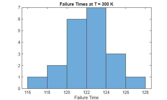
The histogram shows that the failure times at the first stressor level are approximately normally distributed.
Create a plot of mean failure time versus stressor level.
s = groupsummary(failureTable,"T","mean","failureTime");
plot(s.T,s.mean_failureTime,"-o")
xlabel("T")
ylabel("Failure Time");
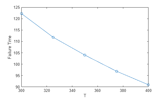
The plot indicates that the mean failure time has a nonlinear dependence on temperature. The failure times in this data set follow an Eyring relationship, which has the functional form f(T) = 1/T*exp(–(b0–b1/T)), where b0 and b1 are model coefficients.
Fit Accelerated Life Model
Fit an accelerated life model to the data using the fitacclife function. Specify a normal life distribution and an Eyring life stress model. Use 230 K as the baseline stressor level.
mdl = fitacclife(failureTable,"failureTime", ...
    Censoring=failureTable.censored,Distribution="normal", ...
    StressModel="eyring",StressorName="T",BaselineStressorLevel=230)
mdl =
AcceleratedLifeModel

Life distribution: normal
Stress model: eyring
Baseline stressor level: 230

     T     NormalMu    MeanFailureTime    AccelerationFactor
    ___    ________    _______________    __________________

    400     90.742         90.742               1.7712
    375     96.951         96.951               1.6577
    350     104.07         104.07               1.5443
    325     112.32         112.32               1.4309
    300     121.99         121.99               1.3175
    230     160.72         160.72                    1


Log-likelihood: -195.5267
mdl is an AcceleratedLifeModel object, which you can use to compute mean failure times, calculate failure probabilities at specific stressor levels, and create plots. The first column of the output contains the unique stressor levels in the data and the baseline stressor level. The second and third columns list the fitted life distribution parameter values and mean failure times, respectively. The fourth column lists the acceleration factor, which is the ratio of the mean failure time at the stressor level to the mean failure time at the baseline stressor level.
Display information about the fitted model coefficients.
mdl.Coefficients
ans=3×3 table
                       Source        Estimate       SE
                   ______________    ________    ________

    b0             "StressModel"     -10.475     0.016919
    b1             "StressModel"      9.8762        5.709
    NormalSigma    "Distribution"     1.7779      0.13054
The table lists the estimated value and the standard error of each coefficient in the life stress model, and the estimated value and the standard error of the life distribution parameter. The life distribution parameter (NormalSigma) and the first coefficient (b0) of the life stress model are well constrained. The second coefficient of the life stress model (b1) is not well constrained.
List the 95% confidence intervals for each fitted model coefficient and parameter.
coefci(mdl)
ans = 3×2

  -10.5084  -10.4412
   -1.4545   21.2070
    1.5188    2.0370
Display the mean failure times according to the model.
meanfailtime(mdl)
ans=6×2 table
     T     MeanFailureTime
    ___    _______________

    400        90.742
    375        96.951
    350        104.07
    325        112.32
    300        121.99
    230        160.72
The last row in the table indicates that the mean failure time at the baseline stressor level (T = 230) is 160.7.
Create a plot of the mean failure times.
meanfailplot(mdl)
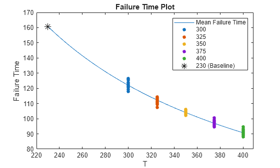
The plot indicates that the Eyring model provides a good fit to the mean failure times at different stressor levels. The mean predicted failure time at the baseline stressor level is indicated on the plot with an asterisk marker.
Create a probability plot of the model and the data.
probplot(mdl)
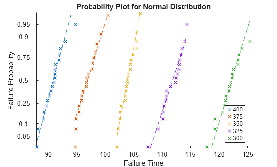
The log-linear plot shows each observation in the data, grouped by stressor level. Each dashed reference line connects the first and third quartiles of the failure time data for that stressor level and extends to the ends of the data. The failure times are shorter at higher temperatures. Also, at a fixed stressor level, the failure probability increases nonlinearly with time.
Load the partFailure data set, which contains simulated observations of failure times for an assembly line part at specific humidity and temperature levels.
load partFailure.matFit an accelerated life model to the data in the partFailure table using the fitacclife function. Use the FailureTime table variable as the failure times, and the other table variables as the stressors.
mdl = fitacclife(partFailure,"FailureTime")mdl =
AcceleratedLifeModel
Life distribution: weibull
Stress model: arrhenius
Humidity Temperature WeibullA MeanFailureTime
________ ___________ ________ _______________
90 35 1.4502 1.3928
90 30 1.5114 1.4516
90 25 1.6015 1.5382
90 20 1.7468 1.6777
90 15 2.0189 1.939
90 12 2.3333 2.241
90 8 3.3507 3.2181
90 5 6.4271 6.1729
80 35 1.4458 1.3886
80 30 1.5069 1.4473
80 25 1.5967 1.5335
80 20 1.7415 1.6727
80 15 2.0128 1.9332
80 12 2.3263 2.2343
80 8 3.3406 3.2084
80 5 6.4077 6.1543
70 35 1.4402 1.3832
70 30 1.501 1.4417
70 25 1.5905 1.5276
70 20 1.7348 1.6662
70 15 2.005 1.9257
70 12 2.3173 2.2256
70 8 3.3276 3.196
70 5 6.3829 6.1304
60 35 1.4328 1.3761
60 30 1.4933 1.4342
60 25 1.5823 1.5197
60 20 1.7259 1.6576
60 15 1.9946 1.9158
60 12 2.3053 2.2141
60 8 3.3104 3.1795
60 5 6.3499 6.0988
50 35 1.4224 1.3662
50 30 1.4825 1.4239
50 25 1.5709 1.5087
50 20 1.7134 1.6456
50 15 1.9803 1.9019
50 12 2.2887 2.1981
50 8 3.2866 3.1566
50 5 6.3041 6.0548
Log-likelihood: 47.0683
mdl is an AcceleratedLifeModel object, which contains information about the fitted model coefficient estimates. By default, the fitacclife function fits an Arrhenius life stress model to the data, and uses a Weibull life distribution. The first and second columns of the displayed output list the unique stressor levels in partFailure. The third and fourth columns list the fitted life distribution parameter values and mean failure times, respectively.
Display information about the fitted model coefficients.
mdl.Coefficients
ans=4×3 table
                    Source        Estimate       SE
                ______________    ________    ________

    b0          "StressModel"      1.1592     0.039112
    b1          "StressModel"     -2.1731       2.0553
    b2          "StressModel"      8.6848      0.11616
    WeibullB    "Distribution"     12.764      0.72011
The table lists the estimated value and the standard error of each coefficient in the life stress model (b0, b1, and b2), and lists the estimated value and the standard error of the life distribution parameter (WeibullB).
List the 95% confidence intervals for each fitted model coefficient and parameter.
ci = coefci(mdl)
ci = 4×2

    1.0819    1.2364
   -6.2330    1.8868
    8.4554    8.9143
   11.3419   14.1867
All the coefficients are well constrained except the b1 coefficient of the Arrhenius life stress model.
Load the partFailure data set, which contains simulated observations of failure times for an assembly line part at specific humidity and temperature levels.
load partFailure.matFit an accelerated life model to the data in the partFailure table using the fitacclife function. Use the FailureTime table variable as the failure times, and the other table variables as the stressors. Set the baseline stressor level to a humidity of 50% and a temperature of 20 degrees Celsius.
mdl = fitacclife(partFailure,"FailureTime",BaselineStressorLevel=[50 20]);Display the mean failure times of the model at each stressor level in the data.
meanfailtime(mdl)
ans=41×3 table
    Humidity    Temperature    MeanFailureTime
    ________    ___________    _______________

       90           35             1.3928
       90           30             1.4516
       90           25             1.5382
       90           20             1.6777
       90           15              1.939
       90           12              2.241
       90            8             3.2181
       90            5             6.1729
       80           35             1.3886
       80           30             1.4473
       80           25             1.5335
       80           20             1.6727
       80           15             1.9332
       80           12             2.2343
       80            8             3.2084
       80            5             6.1543
      ⋮
Create a table of acceleration factors for the unique stressor levels in mdl.
tbl = accelfactor(mdl)
tbl=41×4 table
    Humidity    Temperature    MeanFailureTime    AccelerationFactor
    ________    ___________    _______________    __________________

       90           35             1.3928               1.1815
       90           30             1.4516               1.1336
       90           25             1.5382               1.0699
       90           20             1.6777              0.98087
       90           15              1.939              0.84869
       90           12              2.241              0.73432
       90            8             3.2181              0.51136
       90            5             6.1729              0.26659
       80           35             1.3886               1.1851
       80           30             1.4473               1.1371
       80           25             1.5335               1.0731
       80           20             1.6727              0.98383
       80           15             1.9332              0.85125
       80           12             2.2343              0.73654
       80            8             3.2084              0.51291
       80            5             6.1543               0.2674
      ⋮
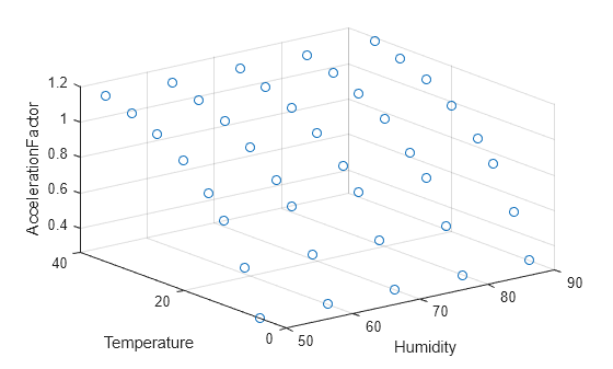
Each acceleration factor is the ratio of the mean failure time at the baseline stressor level to the mean failure time at the stressor level.
Create a 3-D scatter plot showing the acceleration factors of different stressor levels.
scatter3(tbl,"Humidity","Temperature","AccelerationFactor")
Load the partFailure data set, which contains simulated observations of failure times for an assembly line part at specific humidity and temperature levels.
load partFailure.matFit an accelerated life model to the data in the partFailure table using the fitacclife function. Use the FailureTime table variable as the failure times, and the other table variables as the stressors.
mdl = fitacclife(partFailure,"FailureTime");Plot Survivor Function
Return the survivor function values of the model, evaluated at 50 equally spaced time values between 0.8 and 10. By default, the software calculates the survivor function at the lowest unique stressor level in mdl.StressorLevels. In this example, the lowest unique stressor level corresponds to a humidity value of 50% and a temperature of 5 degrees Celsius.
points = linspace(0.8,10,50)';
x = distfcn(mdl,EvaluationTimes=points)
x = 50×1

    0.8000
    0.9878
    1.1755
    1.3633
    1.5510
    1.7388
    1.9265
    2.1143
    2.3020
    2.4898
    2.6776
    2.8653
    3.0531
    3.2408
    3.4286
      ⋮
Plot the survivor function at the evaluation points.
distplot(mdl,EvaluationTimes=points)
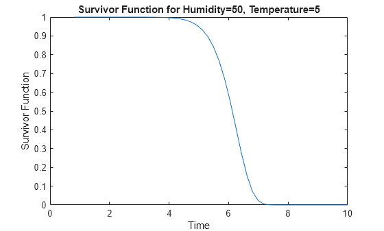
The plot shows that, at this stressor level, the assembly line part has a survival probability close to 100% for time values smaller than 4. The survival probability drops to approximately zero for time values greater than 7.5.
Plot Probability Density Function
Plot the probability density function (pdf).
distplot(mdl,Type="pdf",EvaluationTimes=points)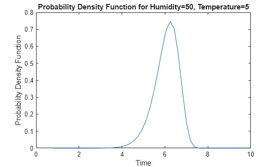
The plot shows that the most likely failure time at this stressor level is approximately 6.2.
Plot Cumulative Distribution Function
Plot the cumulative distribution function (cdf) at a stressor level that corresponds to 90% humidity and a temperature of 20 degrees.
distplot(mdl,[90 20],Type="cdf",EvaluationTimes=points)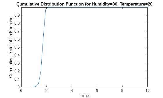
The plot shows that, at this stressor level, approximately half of all assembly line parts have failure times smaller than 1.7.
Plot Inverse Cumulative Distribution Function
Calculate the inverse cumulative distribution function (icdf) at 90% humidity and 35 degrees, and 90% humidity and 20 degrees. Evaluate the icdf at 10 equally spaced probability values between 0.1 and 0.9.
pts = linspace(0.05,0.9,10);
icdfval = [icdf(mdl,pts); icdf(mdl,pts,[90,20])]
icdfval = 2×10

    4.9953    5.4502    5.6944    5.8737    6.0227    6.1562    6.2834    6.4119    6.5525    6.7298
    1.3842    1.5102    1.5779    1.6275    1.6688    1.7058    1.7411    1.7767    1.8156    1.8648
Create a plot of the icdf values for the two stressor levels.
plot(pts,icdfval,"-o")
xlabel("Probability")
ylabel("ICDF Value")
legend(["Humidity = 90, Temperature = 35", ...
    "Humidity = 90, Temperature = 20"],Location="east")
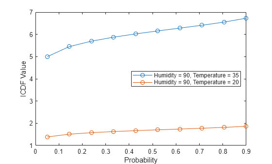
The icdf values are consistently lower at the lower temperature stressor level.
Load the diodeFailure data set, which contains simulated observations of failure times for a diode at different current levels.
load diodeFailure.matFit an accelerated life model to the data in the diodeFailure table using the fitacclife function. Use the FailureTime table variable as the failure times.
mdl = fitacclife(diodeFailure,"FailureTime")mdl =
AcceleratedLifeModel
Life distribution: weibull
Stress model: arrhenius
Current WeibullA MeanFailureTime
_______ ________ _______________
10 1.5323 1.4721
5 2.4956 2.3975
3 4.7821 4.5941
Log-likelihood: 0.4676
mdl is an AcceleratedLifeModel object, which contains information about the fitted model coefficient estimates. By default, the fitacclife function fits an Arrhenius life stress model to the data, using a Weibull life distribution. The first column of the displayed output contains the unique stressor levels in diodeFailure. The second and third columns contain the fitted life distribution coefficient values and mean failure times, respectively.
Create a probability plot.
probplot(mdl)
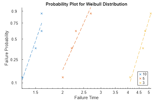
The log-log scatter plot of failure probability versus failure time shows each observation in the data, grouped by stressor level. The dashed lines are linear regression fits to the failure times belonging to each group.
The plot indicates that failure times are shorter at higher current levels, and that the failure probability increases nonlinearly with time at each stressor level.
Load the diodeFailure data set, which contains simulated observations of failure times for a diode at different current levels.
load diodeFailure.matFit an accelerated life model to the data in the diodeFailure table using the fitacclife function. Specify a power law life stress model and use the FailureTime table variable as the failure times.
mdl = fitacclife(diodeFailure,"FailureTime",StressModel="power")
mdl =
AcceleratedLifeModel

Life distribution: weibull
Stress model: power

    Current    WeibullA    MeanFailureTime
    _______    ________    _______________

      10        1.4869           1.41
       5        2.8445         2.6973
       3         4.588         4.3506


Log-likelihood: -3.6697
mdl is an AcceleratedLifeModel object, which contains information about the fitted model coefficient estimates. By default, the fitacclife function uses a Weibull life distribution. The first column of the displayed output lists the unique stressor levels in diodeFailure. The second and third columns list the fitted life distribution values and mean failure times, respectively.
Use the meanfailtime function to compute the predicted mean failure time and the Weibull life distribution parameter at current levels 12 and 15.
[meanFailTimes,lifeCoeffs] = meanfailtime(mdl,[12; 15])
meanFailTimes=2×2 table
    Current    MeanFailureTime
    _______    _______________

      12            1.1888
      15           0.96474
lifeCoeffs=2×2 table
    Current    WeibullA
    _______    ________

      12        1.2537
      15        1.0174
Create a plot of failure time versus current level.
meanfailplot(mdl)
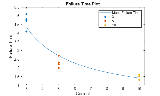
The plot shows that the mean failure time decreases nonlinearly with increasing current level.
More About
Version History
Introduced in R2026a
See Also
fitacclife | accelfactor | coefci | distfcn | distplot | icdf | meanfailplot | meanfailtime | probplot