fitacclife

Fit accelerated life model

Since R2026a

Syntax

mdl = fitacclife(tbl,failureTimeVar)

mdl = fitacclife(tbl,failureTimes)

mdl = fitacclife(tbl,failureTimeInt)

mdl = fitacclife(stressorLevels,failureTimes)

mdl = fitacclife(stressorLevels,failureTimeInt)

mdl = fitacclife(___,Name=Value)

Description

mdl = fitacclife(tbl,failureTimeVar) returns an accelerated life model mdl fit to the data in tbl. The table tbl contains up to two stressor variables and a failure time variable, failureTimeVar, which contains the observed failure times. For more information, see What Is Accelerated Life Analysis?

mdl = fitacclife(tbl,failureTimes) returns the model using the stressor levels in tbl and the observed failure times in the vector failureTimes.

mdl = fitacclife(tbl,failureTimeInt) returns the model using the stressor levels in tbl and the censored failure times in the two-column matrix failureTimeInt.

mdl = fitacclife(stressorLevels,failureTimes) returns the model using the stressor levels in the array stressorLevels and the observed failure times in the vector failureTimes.

mdl = fitacclife(stressorLevels,failureTimeInt) returns the model using the stressor levels in the array stressorLevels and the censoring information in the two-column matrix failureTimeInt.

mdl = fitacclife(___,Name=Value) specifies options using one or more name-value arguments in addition to any of the input argument combinations in the previous syntaxes. For example, StressModel="exponential" specifies to fit the accelerated life model using an exponential life stress model.

Examples

Fit Accelerated Life Model

Load the partFailure data set, which contains simulated observations of failure times for an assembly line part at specific humidity and temperature levels.

load partFailure.mat

Fit an accelerated life model to the data in the partFailure table using the fitacclife function. Use the FailureTime table variable as the failure times, and the other table variables as the stressors.

mdl = fitacclife(partFailure,"FailureTime")

mdl = 
AcceleratedLifeModel

Life distribution: weibull
Stress model: arrhenius

    Humidity    Temperature    WeibullA    MeanFailureTime
    ________    ___________    ________    _______________

       90           35          1.4502         1.3928     
       90           30          1.5114         1.4516     
       90           25          1.6015         1.5382     
       90           20          1.7468         1.6777     
       90           15          2.0189          1.939     
       90           12          2.3333          2.241     
       90            8          3.3507         3.2181     
       90            5          6.4271         6.1729     
       80           35          1.4458         1.3886     
       80           30          1.5069         1.4473     
       80           25          1.5967         1.5335     
       80           20          1.7415         1.6727     
       80           15          2.0128         1.9332     
       80           12          2.3263         2.2343     
       80            8          3.3406         3.2084     
       80            5          6.4077         6.1543     
       70           35          1.4402         1.3832     
       70           30           1.501         1.4417     
       70           25          1.5905         1.5276     
       70           20          1.7348         1.6662     
       70           15           2.005         1.9257     
       70           12          2.3173         2.2256     
       70            8          3.3276          3.196     
       70            5          6.3829         6.1304     
       60           35          1.4328         1.3761     
       60           30          1.4933         1.4342     
       60           25          1.5823         1.5197     
       60           20          1.7259         1.6576     
       60           15          1.9946         1.9158     
       60           12          2.3053         2.2141     
       60            8          3.3104         3.1795     
       60            5          6.3499         6.0988     
       50           35          1.4224         1.3662     
       50           30          1.4825         1.4239     
       50           25          1.5709         1.5087     
       50           20          1.7134         1.6456     
       50           15          1.9803         1.9019     
       50           12          2.2887         2.1981     
       50            8          3.2866         3.1566     
       50            5          6.3041         6.0548     


Log-likelihood: 47.0683

mdl is an AcceleratedLifeModel object, which contains information about the fitted model coefficient estimates. By default, the fitacclife function fits an Arrhenius life stress model to the data, and uses a Weibull life distribution. The first and second columns of the displayed output list the unique stressor levels in partFailure. The third and fourth columns list the fitted life distribution parameter values and mean failure times, respectively.

Display information about the fitted model coefficients.

mdl.Coefficients

ans=4×3 table
                    Source        Estimate       SE   
                ______________    ________    ________

    b0          "StressModel"      1.1592     0.039112
    b1          "StressModel"     -2.1731       2.0553
    b2          "StressModel"      8.6848      0.11616
    WeibullB    "Distribution"     12.764      0.72011

The table lists the estimated value and the standard error of each coefficient in the life stress model (b0, b1, and b2), and lists the estimated value and the standard error of the life distribution parameter (WeibullB).

List the 95% confidence intervals for each fitted model coefficient and parameter.

ci = coefci(mdl)

ci = 4×2

    1.0819    1.2364
   -6.2330    1.8868
    8.4554    8.9143
   11.3419   14.1867

All the coefficients are well constrained except the b1 coefficient of the Arrhenius life stress model.

Visualize Acceleration Factors of Accelerated Life Model

Load the partFailure data set, which contains simulated observations of failure times for an assembly line part at specific humidity and temperature levels.

load partFailure.mat

Fit an accelerated life model to the data in the partFailure table using the fitacclife function. Use the FailureTime table variable as the failure times, and the other table variables as the stressors. Set the baseline stressor level to a humidity of 50% and a temperature of 20 degrees Celsius.

mdl = fitacclife(partFailure,"FailureTime",BaselineStressorLevel=[50 20]);

Display the mean failure times of the model at each stressor level in the data.

meanfailtime(mdl)

ans=41×3 table
    Humidity    Temperature    MeanFailureTime
    ________    ___________    _______________

       90           35             1.3928     
       90           30             1.4516     
       90           25             1.5382     
       90           20             1.6777     
       90           15              1.939     
       90           12              2.241     
       90            8             3.2181     
       90            5             6.1729     
       80           35             1.3886     
       80           30             1.4473     
       80           25             1.5335     
       80           20             1.6727     
       80           15             1.9332     
       80           12             2.2343     
       80            8             3.2084     
       80            5             6.1543     
      ⋮

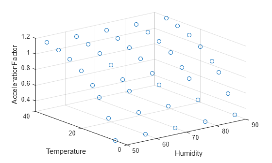
Create a table of acceleration factors for the unique stressor levels in mdl.

tbl = accelfactor(mdl)

tbl=41×4 table
    Humidity    Temperature    MeanFailureTime    AccelerationFactor
    ________    ___________    _______________    __________________

       90           35             1.3928               1.1815      
       90           30             1.4516               1.1336      
       90           25             1.5382               1.0699      
       90           20             1.6777              0.98087      
       90           15              1.939              0.84869      
       90           12              2.241              0.73432      
       90            8             3.2181              0.51136      
       90            5             6.1729              0.26659      
       80           35             1.3886               1.1851      
       80           30             1.4473               1.1371      
       80           25             1.5335               1.0731      
       80           20             1.6727              0.98383      
       80           15             1.9332              0.85125      
       80           12             2.2343              0.73654      
       80            8             3.2084              0.51291      
       80            5             6.1543               0.2674      
      ⋮

Each acceleration factor is the ratio of the mean failure time at the baseline stressor level to the mean failure time at the stressor level.

Create a 3-D scatter plot showing the acceleration factors of different stressor levels.

scatter3(tbl,"Humidity","Temperature","AccelerationFactor")

Input Arguments

tbl — Input data

table

Input data, specified as a table. tbl contains variables for up to two stressors, and can also contain variables for observed or censored failure times. The stressor and failure times variables must be numeric. The allowed stressor data values for specific life stress models depend on the value of the StressModel name-value argument.

• To use table variables that contain stressors and failure times, specify the failureTimeVar input argument. For example, mdl = fitacclife(tbl,"Failure") uses tbl.Failure as the observed failure times, and the remaining columns in tbl as stressor variables.

• To use a subset of table variables as stressors, specify the StressorNames name-value argument. For example, mdl = fitacclife(tbl,"Failure",StressorNames=["Current" "Voltage"]) uses tbl.Current and tbl.Voltage as the stressors, and tbl.Failure as the observed failure times.

• To use table variables that contain censored failure times, censoring indicators, and stressors, specify the failureTimeVar, Censoring, and StressorNames arguments. For example, mdl = fitacclife(tbl,"censoredFailure",Censoring=tbl.censoringIndicators,StressorNames=["Current" "Voltage"]) uses the table variable censoredFailure as the failure times, the table variable censoringIndicators as the censoring indicators, and the table variables Current and Voltage as the stressors. Alternatively, specify the failureTimes and Censoring arguments to use the failure times and censoring indicators contained in workspace variables.

• To use table variables that contain interval-censored failure times and stressors, specify the failureTimeInt input argument and the StressorNames name-value argument. For example, mdl = fitacclife(tbl,[tbl.lowerCens tbl.upperCens],StressorNames=["Stressor1" "Stressor2"]) uses the table variables Stressor1 and Stressor2 as stressor variables, and the table variables lowerCens and upperCens as left-censored and right-censored failure times, respectively. Alternatively, specify the failureTimeInt argument to use the interval-censored failure times contained in a workspace variable.

The variable names in tbl do not have to be valid MATLAB^® identifiers, but the names must not contain leading or trailing blanks. If the names are not valid, you cannot use a formula when you fit or adjust the model.

You can verify the variable names in tbl by using the isvarname function. If the variable names are not valid, then you can convert them by using the matlab.lang.makeValidName function.

failureTimeVar — Name of variable to use as failure times

string scalar | character vector

Name of the variable to use as the failure times, specified as a string scalar or character vector. failureTimeVar indicates which variable in tbl contains the failure time data.

failureTimes — Observed failure times

numeric column vector | duration array

Observed failure times, specified as a numeric column vector or a duration array with n elements, where n is the number of rows in tbl or stressorLevels. Each element in failureTimes corresponds to the same row in tbl or stressorLevels. To specify censored failure times, use the failureTimeInt input argument or the Censoring name-value argument.

Data Types: single | double | duration

failureTimeInt — Interval-censored failure times

two-column numeric matrix

Interval-censored failure times, specified as a two-column numeric matrix with n rows, where n is the number of rows in tbl or stressorLevels. The first and second columns of failureTimeInt contain the lower and upper bounds of the failure times, respectively. Each row corresponds to the same row in tbl or stressorLevels.

• To specify a left-censored failure time, set the lower bound to -Inf.

• To specify a right-censored failure time, set the upper bound to Inf.

• To specify an uncensored failure time, set the upper and lower bounds to the observed failure time value.

stressorLevels — Stressor levels

numeric array

Stressor levels, specified as a numeric array with one or two columns. Each column of stressorLevels contains a stressor in the accelerated life model, and each row contains a stressor level. The allowed values for stressorLevels depend on the life stress model specified by the StressModel name-value argument.

Data Types: single | double

Name-Value Arguments

Specify optional pairs of arguments as Name1=Value1,...,NameN=ValueN, where Name is the argument name and Value is the corresponding value. Name-value arguments must appear after other arguments, but the order of the pairs does not matter.

Example: mdl = fitacclife(tbl,failureTimes,StressModel="exponential") fits an accelerated life model mdl to the stressor levels in tbl and failure times in tbl.failureTimes using an exponential life stress model.

Censoring — Indicator of censored failure times

vector consisting of 0, –1, and 1

Indicator of censored failure times, specified as a vector consisting of 0, –1, and 1, which indicate fully observed, left-censored, and right-censored failure times, respectively. Censoring must have n elements, where n is the number of rows in tbl or stressorLevels. Each element of Censoring indicates the censorship status of the corresponding failure time in failureTimeVar or failureTimes.

You cannot specify interval-censored failure times using this argument. If the sample data includes interval-censored failure times, use the failureTimeInt input argument.

Example: Censoring=censored, where censored is a vector that contains censorship information.

Data Types: logical | single | double

InitialStressModelCoefficients — Initial coefficient estimates of life stress model

numeric vector

Initial coefficient estimates of the life stress model, specified as a numeric vector. InitialStressModelCoefficients must contain n elements, where n is the number of model coefficients in the life stress model specified by StressModel. You must specify InitialStressModelCoefficients when StressModel is a function handle, or when StressModel is "eyring" and the stressor levels and failure times have mixed signs.

Example: InitialStressModelCoefficients=[0.2 0.5 0.6]

Data Types: single | double

InitialDistributionCoefficient — Initial coefficient estimate of life distribution

numeric scalar

Initial coefficient estimate of the life distribution, specified as a numeric scalar. If you specify Distribution="exponential", you cannot specify InitialDistributionCoefficient.

Example: InitialDistributionCoefficient=0.4

Data Types: single | double

StressModel — Life stress model

"arrhenius" (default) | character vector | string scalar | function handle

Life stress model, specified as a function handle or one of the values in the following table, where X1 is the value of the first stressor, X2 is the value of the second stressor (if applicable), and bx are the stress model coefficients. If StressModel is "eyring" and the stressor levels and failure times can have mixed signs, you must also specify InitialStressModelCoefficients.

Value	Life Stress Model	Stressor Data Conditions
"linear"	b0 + b1*X1 + b2*X2	None
"log"	b0 + b1*log(X1) + b2*log(X2)	X1 and X2 must be positive.
"exponential"	b0*exp(b1*X1 + b2*X2)	None
"arrhenius" (default)	b0*exp(b1/X1 + b2/X2)	X1 and X2 must be nonzero.
"power"	b0*X1b1*X2b2	X1 and X2 must be nonnegative.
"reciprocal"	b0 + b1/X1 + b2/X2	X1 and X2 must be nonzero.
"sqrt"	b0 + b1*sqrt(X1) + b2*sqrt(X2)	X1 and X2 must be nonnegative.
"eyring"	(1/X1)*e–(b0 – b1/X1)	X1 and X2 must be nonzero.
"temp-nonthermal"	b0*e-b1/X1*X2b2	X1 must be nonzero, and X2 must be nonnegative.

To specify a custom stress model function, use function handle notation. The function must have this form:

stress = stressFun(X,b)

where X is a one- or two-column matrix of stressor levels, and b is a row vector of model coefficients.

For example, you can define the myFun function as follows, and then specify StressModel as @stressFun.

function stress = stressFun(X,b)
    stress = abs(X(:,1)*b(1) + X(:,2)*b(2));
end

If you specify a custom stress model function, InitialStressModelCoefficients must contain n elements, where n is the number of coefficients in the stress model function.

For more information about life stress models, see What Is Accelerated Life Analysis?

Example: StressModel="eyring"

Data Types: char | string | function handle

Distribution — Life distribution

"weibull" (default) | character vector | string scalar

Life distribution, specified as a character vector or string scalar. The following table shows the supported distributions.

Distribution Name	Distribution Object
"exponential"	ExponentialDistribution
"logistic"	LogisticDistribution
"loglogistic"	LoglogisticDistribution
"lognormal"	LognormalDistribution
"normal"	NormalDistribution
"weibull" (default)	WeibullDistribution

The life distribution is a probability distribution that models the failure time distribution at a specific stressor level. For more information, see What Is Accelerated Life Analysis?

Example: Distribution="normal"

Data Types: char | string

StressorNames — Stressor names

character vector | string array | cell array of character vectors

Stressor names, specified as a character vector, string array, or cell array of character vectors. You can specify one or two stressor names. When you specify stressor levels using the stressorLevels input argument, the length of StressorNames must equal the number of columns in stressorLevels. When you specify input data using the tbl argument, StressorNames must be stressor variable names in tbl.

Example: StressorNames=["Horsepower","Acceleration"]

Data Types: char | string | cell

BaselinestressorLevel — Baseline stressor level

numeric vector

Baseline stressor level, specified as a numeric vector. The length of BaselinestressorLevel must equal the number of stressors in tbl or stressorLevels.

Example: BaselinestressorLevel=[20 40]

Data Types: single | double

Options — Optimization options

statset("fitacclife") (default) | structure

Optimization options, specified as a structure. This argument determines the control parameters for the iterative algorithm used by fitacclife.

Create optimization options by using the statset function or by creating a structure array containing the following fields.

Field Name	Description	Default Value
FunValCheck	Flag indicating whether fitacclife checks the values returned by the distribution functions for validity, specified as "on" or "off". A poor choice for the starting point can cause the distribution functions to return NaNs, infinite values, or out-of-range values if you define the function without suitable error checking.	"on"
TolFun	Termination tolerance on the function value, specified as a positive scalar.	1e-6
TolX	Termination tolerance for the parameters, specified as a positive scalar.	1e-6
MaxFunEvals	Maximum number of function evaluations allowed, specified as a positive integer.	1000
MaxIter	Maximum number of iterations allowed, specified as a positive integer.	1000
Display	Level of display, specified as "off", "final", or "iter". "off" — Display no information. "final" — Display the final information. "iter" — Display information at each iteration.	"off"

You can also enter statset("fitacclife") in the Command Window to display the default value of each option.

When you specify an option, you can preserve the default values for all other options by additionally specifying statset("fitacclife"). For example, statset(statset("fitacclife"), MaxIter=1000) sets the maximum number of iterations to 1000, and uses the default values for all other options.

Example: Options=statset(MaxIter=2000,TolX=1e-7) specifies to use a maximum of 2000 iterations and a termination tolerance of 1e-7.

Data Types: struct

Output Arguments

mdl — Accelerated life model

AcceleratedLifeModel object

Accelerated life model, returned as an AcceleratedLifeModel object. For properties and functions of this object, see AcceleratedLifeModel.

Version History

Introduced in R2026a