What Is Accelerated Life Analysis?

Accelerated life analysis provides a way to predict the lifetimes of industrial components when you cannot directly obtain time-to-failure data under normal operating conditions. For example, the mean lifetime of a light bulb might be much longer than the feasible timescale for an experimental study. By gathering failure time data on a component when it is subjected to abnormal stressor levels, such as high or low ambient temperature or humidity, you can model the component's lifetime characteristics and determine quantities such as the failure rate and mean failure time under normal operating conditions.

The typical steps in accelerated life analysis are:

1. Identify one or more stressors that have the strongest impact on the component's lifetime.

2. Construct an experiment, for example, using Design of Experiments (DOE) techniques, to measure failure times at different stressor levels.

3. Choose a Life Distribution that best represents the failure rate characteristics of the component.

4. Choose a Life Stress Model that best describes the mean failure time of the component at different stressor levels.

5. Create an accelerated life model by fitting the life distribution and stress model to the failure time data.

6. Use the fitted accelerated life model to predict the lifetime characteristics of the component under normal operating conditions.

You can perform accelerated life analysis in Statistics and Machine Learning Toolbox™ by creating an AcceleratedLifeModel model object using the fitacclife function. For an example, see Perform Accelerated Life Model Analysis.

Censoring

In accelerated life analysis, censoring occurs when the failure times of some components are not fully observed due to different reasons. Right-censoring can occur if a component does not fail before the end of the reliability study. Alternatively, a failure time can be left-censored if the failure is observed only at some time after its actual occurrence.

When you perform accelerated life analysis with Statistics and Machine Learning Toolbox, you can specify censored failure times by using a vector of indicator variables for left- or right-censoring, or by specifying failure time intervals as an array of lower and upper bounds.

The following table shows a simulated set of failure times of components subjected to one of three stressor levels in a 25-week study. Two of the failure times are right-censored (censoring indicator = 1). These components did not fail by the end of the study. One failure time is left-censored (censoring indicator = –1) because the component failure was not noticed until the 20th week of the study. The fourth column of the table lists the failure times in censoring interval format.

Stressor Level	Failure Time (Weeks)	Censoring Indicator	Censoring Interval
2	14	0	[14 14]
1	23	0	[23 23]
3	7	0	[7 7]
1	25	1	[25 Inf]
2	19	0	[19 19]
2	16	0	[16 16]
1	25	1	[25 Inf]
1	20	–1	[–Inf 20]

Life Distribution

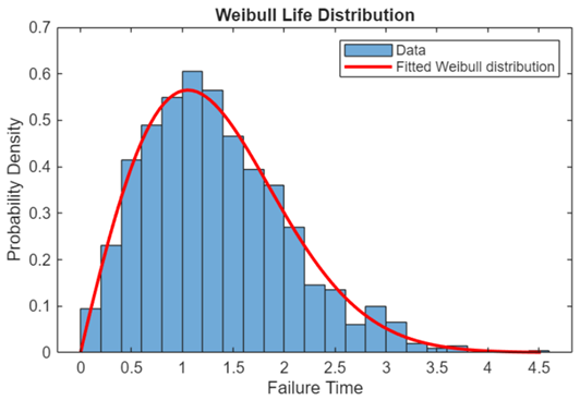
A life distribution is a probability distribution that models the failure time distribution of a component at a fixed stressor level. Depending on the processes that influence when component failure occurs, the life distribution can have many forms, such as exponential, logistic, or normal. In cases where the main cause of component failure is wear or material fatigue, the probability of failure typically rises sharply at first, reaches a peak, and then declines exponentially over time. For this reason, a commonly used life distribution is the Weibull Distribution, whose shape is determined by two parameters a and b. The following figure shows a set of failure times fit by a Weibull distribution with a = 1.5 and b = 2.

Life Stress Model

A life stress model is a function that describes the mean failure time of a component at different stressor levels. The functional form of a life stress model depends on the details of the failure process. Some commonly used stress models are:

• Arrhenius, for processes involving temperature-related stressors

• Eyring, for processes involving temperature and additional stressors

• Exponential, for processes involving nonthermal stressors

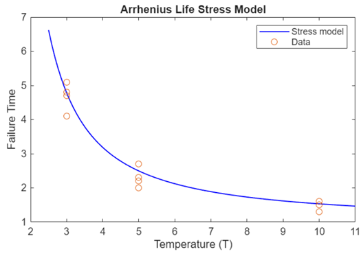
The following figure shows a set of failure times fit by an Arrhenius distribution, which has the functional form f(T) = a*exp(b/T), where T is the stressor value and a and b are the model coefficients.

Accelerated Life Model Analysis

To create an accelerated life model, fit a life distribution and a life stress model to a failure time data set. You can use an accelerated life model to:

• Estimate the mean failure time at a baseline stressor level that corresponds to normal operating conditions.

• Compute the survivor and failure rate functions over time at the baseline stressor level or other stressor levels.

• Compute acceleration factors. An acceleration factor is the ratio of the mean failure time at the baseline stressor level to the mean failure time at a specified stressor level.

For an example of an accelerated life model analysis workflow, see Accelerated Life Model Analysis.

References

[1] Nelson, Wayne. Accelerated Testing: Statistical Models, Test Plans and Data Analyses. Wiley Series in Probability and Mathematical Statistics. New York: Wiley, 1990.