Compute Envelope Spectrum of Vibration Signal
Use Signal Analyzer to compute the envelope spectrum of a bearing vibration signal and look for defects. Generate MATLAB® scripts and functions to automate the analysis.
Generate Bearing Vibration Data
A bearing with the dimensions shown in the figure is driven at cycles per second. An accelerometer samples the bearing vibrations at 10 kHz.
Generate vibration signals from two defective bearings using the bearingdata function at the end of the example. In one of the signals, xBPFO, the bearing has a defect in the outer race. In the other signal, xBPFI, the bearing has a defect in the inner race. For more details on modeling and diagnosing defects in bearings, see Vibration Analysis of Rotating Machinery and envspectrum.
[t,xBPFO,xBPFI,bpfi] = bearingdata;
Compute Envelope Spectrum Using Signal Analyzer
Open Signal Analyzer and drag the BPFO signal to a display. Add time information to the signal by selecting it in the Signal table and clicking Time Values on the Analyzer tab. Select Sample Rate and Start Time and enter 10 kHz for the sample rate.
On the Display tab, click Spectrum to open a spectrum view. The spectrum of the vibration signal shows BPFO harmonics modulated by 3 kHz, which corresponds to the impact frequency specified in bearingdata. At the low end of the spectrum, the driving frequency and its orders obscure other features.

Select the signal and, on the Analyzer tab, click Duplicate to generate a copy of it. Give the new signal the name envspec and drag it to the display. Compute the envelope spectrum of the signal using the Hilbert transform. Select envspec in the Signal table and click Preprocess to enter the preprocessing mode.
Remove the DC value of the signal. In the Functions gallery, select Detrend. In the Function Parameters panel, select
Constantas the detrend method. Click Apply.Bandpass-filter the detrended signal. In the Functions gallery, select Bandpass. In the Function Parameters panel, enter
2250 Hzand3750 Hzas the lower and upper passband frequencies, respectively. Click Apply.Compute the envelope of the filtered signal. In the Functions gallery, select Envelope. In the Function Parameters panel, select
Hilbertas the method. Click Apply.Remove the DC value of the envelope. In the Functions gallery, select Detrend. In the Function Parameters panel, select
Constantas the detrend method. Click Apply.
Click the icon in the Info column to view the preprocessing information.

Click Accept All to save the preprocessing results and exit the mode. The envelope spectrum appears in the spectrum view of the display. The envelope spectrum clearly displays the BPFO harmonics.

Steps to Create an Integrated Analysis Script
The computation of the envelope spectrum can get tedious if it has to be repeated for many different bearings. Signal Analyzer can generate MATLAB® scripts and functions to help you automate the computation.
As an exercise, repeat the previous analysis for the BPFI signal. Signal Analyzer generates two components useful for the automation:
preprocess, a function that preprocesses the signal by detrending it, filtering it, and computing its envelopeCompute power spectrum, a script that computes the envelope spectrum
To create the integrated analysis script, put the preprocessing function and the plotting script together unchanged in a single file. (Alternatively, you can save functions in separate files.)
If you save the script and the function in a single MATLAB® script, keep in mind that functions must appear at the end.
You must add the keyword
endat the end of each function.
1. Create Preprocessing Function
Initially, create the function that reproduces the preprocessing steps. Select the envspec signal. On the Analyzer tab, click Generate Function. The function, called preprocess by default, appears in the Editor. Save the generated function at the end of your integrated analysis script. The function expects a second argument specifying the time information. Preprocess the BPFI signal using the function.
envspec = preprocess(xBPFI,t);
2. Create Spectrum Script
In the app, remove the unprocessed signal from the display by clearing the check box next to its name. On the Display tab, click Generate Script and select Spectrum Script. The script appears in the Editor. Include the generated code in your integrated analysis script. When you run the analysis script, the generated spectrum script computes the envelope spectrum of the preprocessed BPFI signal.
% Compute power spectrum

% Generated by MATLAB(R) 9.6 and Signal Processing Toolbox 8.2.
% Generated on: 12-Nov-2018 15:13:34

% Parameters
timeLimits = [0 0.9999]; % seconds
frequencyLimits = [0 5000]; % Hz

%%
% Index into signal time region of interest
envspec_ROI = envspec(:);
sampleRate = 10000; % Hz
startTime = 0; % seconds
minIdx = ceil(max((timeLimits(1)-startTime)*sampleRate,0)) + 1;
maxIdx = floor(min((timeLimits(2)-startTime)*sampleRate, ...
    length(envspec_ROI)-1)) + 1;
envspec_ROI = envspec_ROI(minIdx:maxIdx);

% Compute spectral estimate. To plot the results,
% run the function call below without output arguments.
[Penvspec_ROI, Fenvspec_ROI] = pspectrum(envspec_ROI,sampleRate, ...
    FrequencyLimits=frequencyLimits);
3. Plot Envelope Spectrum
Plot the envelope spectrum. Compare the peak locations to the frequencies of the first ten BPFI harmonics. You can also plot the envelope spectrum using the pspectrum command with no output arguments.
plot(Fenvspec_ROI,(Penvspec_ROI))
xline((1:10)*bpfi,":")
xlim([0 10*bpfi])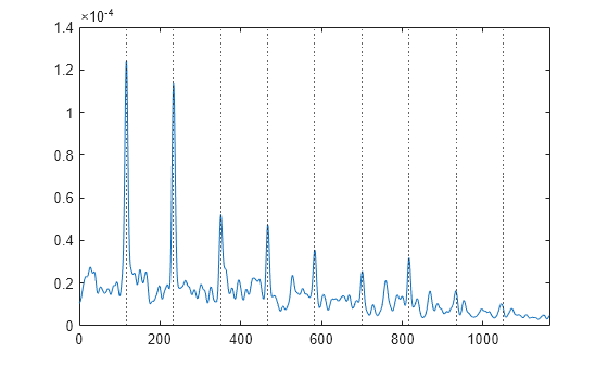
Function Code
Signal Preprocessing Function
The signal preprocessing function generated by the app combines detrending, bandpass filtering, and envelope computation.
function y = preprocess(x,tx)
%  Preprocess input x
%    This function expects an input vector x and a vector of time values
%    tx. tx is a numeric vector in units of seconds.

% Generated by MATLAB(R) 9.6 and Signal Processing Toolbox 8.2.
% Generated on: 12-Nov-2018 15:09:44

y = detrend(x,"constant");
Fs = 1/mean(diff(tx)); % Average sample rate
y = bandpass(y,[2250 3750],Fs,Steepness=0.85,StopbandAttenuation=60);
[y,~] = envelope(y);
y = detrend(y,"constant");
end
Bearing Data Generating Function
The bearing has pitch diameter cm and a bearing contact angle . Each of the rolling elements has a diameter cm. The outer race remains stationary as the inner race is driven at cycles per second. An accelerometer samples the bearing vibrations at 10 kHz.
function [t,xBPFO,xBPFI,bpfi] = bearingdata

p = 0.12;
d = 0.02;
n = 8;
th = 0;
f0 = 25;
fs = 10000;
For a healthy bearing, the vibration signal is a superposition of several orders of the driving frequency, embedded in white Gaussian noise.
t = 0:1/fs:1-1/fs;
z = [1 0.5 0.2 0.1 0.05]*sin(2*pi*f0*[1 2 3 4 5]'.*t);

xHealthy = z + randn(size(z))/10;
A defect in the outer race causes a series of 5 millisecond impacts that over time result in bearing wear. The impacts occur at the ball pass frequency outer race (BPFO) of the bearing,
.
Model the impacts as a periodic train of 3 kHz exponentially damped sinusoids. Add the impacts to the healthy signal to generate the BPFO vibration signal.
bpfo = n*f0/2*(1-d/p*cos(th));

tmp = 0:1/fs:5e-3-1/fs;
xmp = sin(2*pi*3000*tmp).*exp(-1000*tmp);

xBPFO = xHealthy + pulstran(t,0:1/bpfo:1,xmp,fs)/4;
If the defect is instead in the inner race, the impacts occur at a frequency
.
Generate the BPFI vibration signal by adding the impacts to the healthy signals.
bpfi = n*f0/2*(1+d/p*cos(th));

xBPFI = xHealthy + pulstran(t,0:1/bpfi:1,xmp,fs)/4;

end
See Also
Apps
Functions
Topics
- Find Delay Between Correlated Signals
- Resolve Tones by Varying Window Leakage
- Compute Signal Spectrum Using Different Windows
- Find Interference Using Persistence Spectrum
- Modulation and Demodulation Using Complex Envelope
- Find and Track Ridges Using Reassigned Spectrogram
- Extract Voices from Music Signal
- Resample and Filter a Nonuniformly Sampled Signal
- Declip Saturated Signals Using Your Own Function
- Extract Regions of Interest from Whale Song
- Use Signal Analyzer App
- Edit Sample Rate and Other Time Information
- Data Types Supported by Signal Analyzer
- Spectrum Computation in Signal Analyzer
- Persistence Spectrum in Signal Analyzer
- Spectrogram Computation in Signal Analyzer
- Scalogram Computation in Signal Analyzer
- Keyboard Shortcuts for Signal Analyzer
- Signal Analyzer Tips and Limitations