Resample and Filter a Nonuniformly Sampled Signal
A person recorded their weight in pounds during the leap year 2012. The person did not record their weight every day, so the data are nonuniform. Use the Signal Analyzer app to preprocess and study the recorded weight. The app enables you to fill in the missing data points by interpolating the signal to a uniform grid. (This procedure gives the best results if the signal has only small gaps.)
Load the data and convert the measurements to kilograms. The data file has the missing readings set to NaN. There are 27 data points missing, most of them during a two-week stretch in August.
wt = datetime(2012,1,1:366)';

load weight2012.dat
wgt = weight2012(:,2)/2.20462;

validpoints = ~isnan(wgt);
missing = wt(~validpoints);
missing(15:26)
ans = 12×1 datetime
09-Aug-2012
10-Aug-2012
11-Aug-2012
12-Aug-2012
15-Aug-2012
16-Aug-2012
17-Aug-2012
18-Aug-2012
19-Aug-2012
20-Aug-2012
22-Aug-2012
23-Aug-2012
Store the data in a MATLAB® timetable. Remove the missing points. Remove the DC value to concentrate on fluctuations. Convert the time information to a duration array by subtracting the first time point. For more details, see Data Types Supported by Signal Analyzer.
wgt = wgt(validpoints);
wgt = wgt - mean(wgt);

wt = wt(validpoints);
wt = wt - wt(1);

wg = timetable(wt,wgt);
Open Signal Analyzer and drag the timetable to a display. On the Display tab, click Spectrum to open a spectrum view. On the Time tab, select Show Markers. Zoom into the missing stretch by setting the Time Limits to 200 and 250 days.

Right-click the signal in the Signal table and select Duplicate. Rename the copy as Preprocessed by right-clicking the signal in the Signal table and selecting Rename. Select the preprocessed signal in the Signal table and, on the Analyzer tab, click Preprocess. In the Functions gallery, select Resample. In the Function Parameters panel that appears, specify these parameters:
Resampling Method —
Sample RateFrequency Units —
cycles/daySample Rate —
1Interpolation Method —
Shape Preserving Cubicmethod
Click Apply and then click Accept All to save the results and exit the preprocessing mode. Overlay the resampled signal on the display by selecting the check box next to its name.

Zoom out to reveal the data for the whole year. On the Spectrum tab, set the leakage to the maximum value. The spectra of the original and resampled signals agree well for most frequencies. The spectrum shows two noticeable peaks, one at around 0.14 cycles/day and the other at very low frequencies. To locate the peaks better, on the Display tab, click Data Cursors and select Two. Place the cursors on the peaks. Hover over the frequency field of each cursor to get a more precise value of its location.
The medium-frequency peak is at 0.143 = 1/7 cycles/day, which corresponds to a one-week cycle.
The low-frequency peak is at 0.005 cycles/day, which corresponds to a 210-day cycle.

Remove the cursors by clicking Data Cursors. Remove the original signal from the display. Filter the Preprocessed signal to remove the effects of the cycles. With the preprocessed signal selected in the Signal Table, on the Analyzer tab, click Preprocess. Inside the preprocessing mode:
To remove the low-frequency cycle, highpass-filter the signal. Select Highpass from the Functions gallery. In the Function Parameters panel that appears, enter a passband frequency of
0.05 cycles/day. Use the default values of the other parameters. Click Apply.To remove the weekly cycle, bandstop-filter the signal. Select Bandstop from the Functions gallery. In the Function Parameters panel, enter a lower passband frequency of
0.135 cycles/dayand a higher passband frequency of0.15 cycles/day. Use the default values of the other parameters. Click Apply.
Inspect the results and click Accept All. Plot both signals in the display.

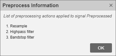
The preprocessed signal shows less fluctuation than the original. The shape of the signal suggests the person's weight varies less in the summer months than in winter, but that may be an artifact of the resampling. Click the icon on the Info column in the Signal table entry for the Preprocessed signal to see the preprocessing steps performed on it.
To see a full summary of the preprocessing steps, including all the settings you chose, click Generate Function on the Analyzer tab. The generated function appears in the MATLAB® Editor.
function [y,ty] = preprocess(x,tx)
%  Preprocess input x
%    This function expects an input vector x and a vector of time values
%    tx. tx is a numeric vector in units of seconds.
%    Follow the timetable documentation (type 'doc timetable' in
%    command line) to learn how to index into a table variable and its time
%    values so that you can pass them into this function.

% Generated by MATLAB(R) 9.13 and Signal Processing Toolbox 9.0.
% Generated on: 03-Jan-2022 15:47:27

targetSampleRate = 1.1574074074074073e-05;
[y,ty] = resample(x,tx,targetSampleRate,'pchip');

Fs = 1/mean(diff(ty)); % Average sample rate
y = highpass(y,5.787e-07,Fs,'Steepnes',0.85,'StopbandAttenuation',60);

y = bandstop(y,[1.5625e-06 1.73611111111111e-06],Fs,'Steepness',0.85,'StopbandAttenuation',60);
end
See Also
Apps
Functions
Topics
- Find Delay Between Correlated Signals
- Resolve Tones by Varying Window Leakage
- Compute Signal Spectrum Using Different Windows
- Find Interference Using Persistence Spectrum
- Modulation and Demodulation Using Complex Envelope
- Find and Track Ridges Using Reassigned Spectrogram
- Extract Voices from Music Signal
- Declip Saturated Signals Using Your Own Function
- Compute Envelope Spectrum of Vibration Signal
- Extract Regions of Interest from Whale Song
- Use Signal Analyzer App
- Edit Sample Rate and Other Time Information
- Data Types Supported by Signal Analyzer
- Spectrum Computation in Signal Analyzer
- Persistence Spectrum in Signal Analyzer
- Spectrogram Computation in Signal Analyzer
- Scalogram Computation in Signal Analyzer
- Keyboard Shortcuts for Signal Analyzer
- Signal Analyzer Tips and Limitations