receive
Syntax
Description
RXsig = receive(RX,TXsig,TXinfo,propPaths)RX, where
TXsig is the transmitted signal returned by the
transmit function called on the bistaticTransmitter
object. On each call to receive, the transmissions defined by
TXsig are propagated to RX and received.
Received signals that lie between the current simulation time and the simulation time at the
previous call to receive are returned. The simulation time is updated
to the start time of the transmitted signal specified in TXinfo. Ensure
that all of the possible transmissions for the current receive window are included by
calling receive when the simulation has reached the start of the next
receive window. You can get the start time for the next receive window by calling nextTime on
RX.
[___] = receive(
returns signals received by the bistatic receiver object, RX,propSig,propInfo)RX, where
propSig is the coherently combined transmitted signal returned by
collect. The ability to receive after collect is
called on RX allows multiple transmissions to be collected and
coherently combined between calls to receive. You can use this syntax
when multiple repetition intervals of a transmitted waveform need to be received.
Examples
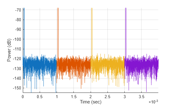
This example shows how to create a simple bistatic scenario with a moving target. Transmit and collect pulses until the completion of 1 receive window and plot the results.
Configure the bistatic transmitter and receiver. Use a pulse repetition frequency of 1000 Hz.
prf   = 1e3;
wav   = phased.LinearFMWaveform(PRF=prf,PulseWidth=1e-5);
ant   = phased.SincAntennaElement(Beamwidth=10);
tx    = bistaticTransmitter(Waveform=wav, ...
      Transmitter=phased.Transmitter(Gain=20), ...
      TransmitAntenna=phased.Radiator(Sensor=ant));
rx    = bistaticReceiver( ...
      ReceiveAntenna=phased.Collector(Sensor=ant), ...
      WindowDuration=0.005);
freq  = tx.TransmitAntenna.OperatingFrequency;
Create bistatic transmitter and bistatic receiver platforms spaced 10 km apart and add a target platform. Use radarScenario to create the platforms for this example. Define the transmitter platform, receiver platform, and target platform using platform and give the target a trajectory.
scene  = radarScenario(UpdateRate=prf);
platform(scene,Position=[-5e3 0 0], ...
       Orientation=rotz(45).');
platform(scene,Position=[5e3 0 0], ...
       Orientation=rotz(135).');
traj   = kinematicTrajectory( ...
       Position=8e3*[cosd(60) sind(60) 0],Velocity=[0 150 0]);
tgtPlat= platform(scene,Trajectory=traj);
Create an empty plot.
hFig  = figure;
hAxes = axes(hFig);
Transmit and collect pulses for one receive window. First, update platform positions by calling advance on the scene and then get the platform positions using platformPoses. Next, get the propagation paths using bistaticFeeSpacePath. Then, transmit the signal and receive pulses. Finally, plot the received signals.
t    = nextTime(tx);
tEnd = nextTime(rx);
while t < tEnd
    advance(scene);
    % Get platform positions
    poses = platformPoses(scene);

    % Calculate paths
    proppaths = bistaticFreeSpacePath(freq, ...
              poses(1),poses(2),poses(3));

    % Transmit
    [txSig,txInfo] = transmit(tx,proppaths,t);

    % Receive pulses
    [iq,rxInfo] = receive(rx,txSig,txInfo,proppaths);
    t = nextTime(tx);

    % Plot received signals
    rxTimes = (0:(size(iq,1) - 1))*1/rxInfo.SampleRate ...
            + rxInfo.StartTime;
    plot(hAxes,rxTimes,mag2db(abs(sum(iq,2))))
            hold(hAxes,'on')
end
Label the plot.
grid(hAxes,'on')
xlabel(hAxes,'Time (sec)')
ylabel(hAxes,'Power (dB)')
axis(hAxes,'tight')
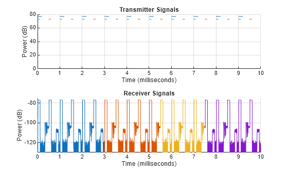
This example shows how to create a bistatic scenario with two bistatic transmitters. The receiver is located between the transmitters and there is a target with a custom radar cross section. Transmit and collect pulses for four receive windows and plot the results.
Configure the bistatic transmitters. Use a pulse repetition frequency of 1000 Hz.
prf   = 1e3;
wav   = phased.LinearFMWaveform(PRF=prf,PulseWidth=0.2/prf);
ant   = phased.SincAntennaElement(Beamwidth=10);
tx1   = bistaticTransmitter(Waveform=wav, ...
      Transmitter=phased.Transmitter(Gain=40), ...
      TransmitAntenna=phased.Radiator(Sensor=ant));
tx2   = clone(tx1);
prf   = 2e3;
tx2.Waveform = phased.RectangularWaveform( ...
      PRF=prf,PulseWidth=0.2/prf);
tx2.Transmitter.PeakPower = 2e3;
Configure the bistatic receiver.
rx    = bistaticReceiver( ...
      ReceiveAntenna=phased.Collector(Sensor=ant), ...
      WindowDuration=0.0025);
freq  = tx1.TransmitAntenna.OperatingFrequency;
Create bistatic transmitter platforms spaced 10 km apart. Put the receiver platform between the two transmitters. For this example, create the platforms in radarScenario. Define the platforms using platform.
scene   = radarScenario(UpdateRate=prf);
tx1Plat = platform(scene,Position=[-5e3 0 0], ...
        Orientation=rotz(85).');
tx2Plat = platform(scene,Position=[5e3 0 0], ...
        Orientation=rotz(95).');
rxPlat  = platform(scene,Position=[0 0 0], ...
        Orientation=rotz(90).');
Place a stationary target platform down range and assign the target a radar cross section.
rcsSig = rcsSignature(Pattern=20);
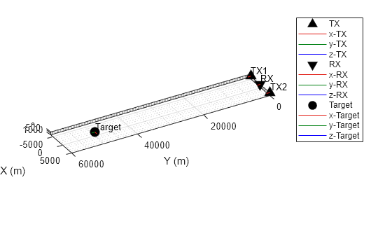
tgtPlat = platform(scene,Position=[0 50e3 0], ...
Signatures=rcsSig);Show platform locations and orientations.
tp     = theaterPlot(Parent=axes(figure));
txPltr = orientationPlotter(tp,Marker="^", ...
       DisplayName="TX",LocalAxesLength=1e3);
rxPltr = orientationPlotter(tp,Marker="v", ...
       DisplayName="RX",LocalAxesLength=1e3);
tgtPltr = orientationPlotter(tp,Marker="o", ...
        DisplayName="Target",LocalAxesLength=1e3);
poses   = platformPoses(scene);
plotOrientation(txPltr,[poses(1:2).Orientation], ...
reshape([poses(1:2).Position],3,[]).',["TX1" "TX2"]);
plotOrientation(rxPltr,poses(3).Orientation,poses(3).Position,"RX");
plotOrientation(tgtPltr,poses(4).Orientation,poses(4).Position,"Target");
Transmit and collect pulses for four receive windows. First, update platform positions by calling advance on the scene. Then set up the for loop to iterate over the receive windows. Next, get platform positions using platformPoses. Get the propagation paths for both transmitters using bistaticFeeSpacePath. Then, transmit the signal and collect pulses. Finally, receive the transmissions and plot the received signals.
tl    = tiledlayout(figure,2,1);
hAxes = [nexttile(tl) nexttile(tl)]; hold(hAxes,"on");
tx    = {tx1 tx2};
advance(scene);
for iRxWin = 0:4
    [propSigs,propInfo] = collect(rx,scene.SimulationTime);
    t    = min([nextTime(tx{1}) nextTime(tx{2})]);
    tEnd = nextTime(rx);
    while t <= tEnd
        % Get platform positions
        poses = platformPoses(scene);

        % Include target RCS signature on the pose
        tgtPose   = poses(4);
        tgtPose.Signatures = {rcsSig};

        for iTx = 1:2
            % Calculate propogation paths
            proppaths = bistaticFreeSpacePath(freq, ...
                      poses(iTx),poses(3),tgtPose);

            % Transmit
            [txSig,txInfo] = transmit(tx{iTx},proppaths,scene.SimulationTime);

            % Plot transmitted signal
            txTimes = (0:(size(txSig,1) - 1))*1/txInfo.SampleRate ...
                    + txInfo.StartTime;
            plot(hAxes(1),txTimes*1e3,mag2db(max(abs(txSig),[],2)),SeriesIndex=iTx);

            % Collect transmitted pulses
            collectSigs = collect(rx,txSig,txInfo,proppaths);

            % Accumulate collected transmissions
            sz = max([size(propSigs);size(collectSigs)],[],1);
            propSigs = paddata(propSigs,sz) + paddata(collectSigs,sz);
         end

         t = min([nextTime(tx{1}) nextTime(tx{2})]);
         advance(scene);
    end


    % Receive collected transmissions
    [iq,rxInfo] = receive(rx,propSigs,propInfo);

    % Plot received transmissions
    rxTimes = (0:(size(iq,1) - 1))*1/rxInfo.SampleRate ...
            + rxInfo.StartTime;
    plot(hAxes(2),rxTimes*1e3,mag2db(abs(iq)));
end
Label plots.
grid(hAxes,"on")
title(hAxes(1),"Transmitter Signals")
title(hAxes(2),"Receiver Signals")
xlabel(hAxes,"Time (milliseconds)")
ylabel(hAxes,"Power (dB)")
ylim(hAxes(1),[0 80]); ylim(hAxes(2),[-130 -75])
xlim(hAxes(1),xlim(hAxes(2)))
This example shows how to create a simple bistatic scenario with a moving target. Transmit and collect pulses until the completion of 1 receive window and plot the results.
Configure the bistatic transmitter and receiver. Use a pulse repetition frequency of 1000 Hz.
prf   = 1e3;
wav   = phased.LinearFMWaveform(PRF=prf,PulseWidth=1e-5);
ant   = phased.SincAntennaElement(Beamwidth=10);
tx    = bistaticTransmitter(Waveform=wav, ...
      Transmitter=phased.Transmitter(Gain=20), ...
      TransmitAntenna=phased.Radiator(Sensor=ant));
rx    = bistaticReceiver( ...
      ReceiveAntenna=phased.Collector(Sensor=ant), ...
      WindowDuration=0.005);
freq  = tx.TransmitAntenna.OperatingFrequency;
Create bistatic transmitter and bistatic receiver platforms spaced 10 km apart and add a target platform. Use radarScenario to create the platforms for this example. Define the transmitter platform, receiver platform, and target platform using platform and give the target a trajectory.
scene  = radarScenario(UpdateRate=prf);
platform(scene,Position=[-5e3 0 0], ...
       Orientation=rotz(45).');
platform(scene,Position=[5e3 0 0], ...
       Orientation=rotz(135).');
traj   = kinematicTrajectory( ...
       Position=8e3*[cosd(60) sind(60) 0],Velocity=[0 150 0]);
tgtPlat= platform(scene,Trajectory=traj);
Create an empty plot.
hFig  = figure;
hAxes = axes(hFig);
Transmit and collect pulses for one receive window. First, update platform positions by calling advance on the scene and then get the platform positions using platformPoses. Next, get the propagation paths using bistaticFeeSpacePath. Then, transmit the signal and receive pulses. Finally, plot the received signals.
t    = nextTime(tx);
tEnd = nextTime(rx);
while t < tEnd
    advance(scene);
    % Get platform positions
    poses = platformPoses(scene);

    % Calculate paths
    proppaths = bistaticFreeSpacePath(freq, ...
              poses(1),poses(2),poses(3));

    % Transmit
    [txSig,txInfo] = transmit(tx,proppaths,t);

    % Receive pulses
    [iq,rxInfo] = receive(rx,txSig,txInfo,proppaths);
    t = nextTime(tx);

    % Plot received signals
    rxTimes = (0:(size(iq,1) - 1))*1/rxInfo.SampleRate ...
            + rxInfo.StartTime;
    plot(hAxes,rxTimes,mag2db(abs(sum(iq,2))))
            hold(hAxes,'on')
end
Label the plot.
grid(hAxes,'on')
xlabel(hAxes,'Time (sec)')
ylabel(hAxes,'Power (dB)')
axis(hAxes,'tight')
Input Arguments
Output Arguments
Version History
Introduced in R2025a