Parallel Simulation of Target, Clutter, and Interference Signals

Since R2025a

This example shows how to model clutter and interference for a monostatic radar. You will use bistaticTransmitter and bistaticReceiver to model both halves of a monostatic radar. You will see how these features enable you to:

• Speed up the processing for large clutter scenarios by using parfor

• Inject interference signals into a monostatic radar's receiver

You will also use spatial and Doppler notch filters to recover the desired target detections in the presence of strong interference and clutter signals.

Define the Scenario

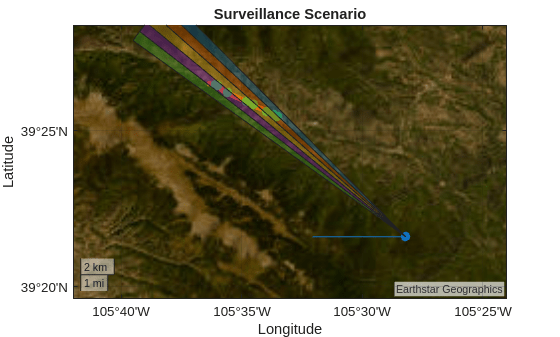
Set up a simulation of an airborne radar to monitor traffic conditions on a mountain road. Use digital terrain elevation data (DTED) and insert cars to make the simulation realistic. To start, show the portion of the road being monitored by the radar. Save the handle to the new figure so that you can continue updating it later in the example.

figScene = figure;
geobasemap streets
geolimits([39.35 39.45],[-105.7 -105.4])
hold on
rng default % Set random seed for repeatable results

Use the helperAreaOfInterest function to retrieve the latitude and longitude waypoints for the area of interest along the road.

[roadLats,roadLons] = helperAreaOfInterest;
geoplot(roadLats,roadLons,SeriesIndex=2,LineWidth=4)
title("Surveillance Scenario")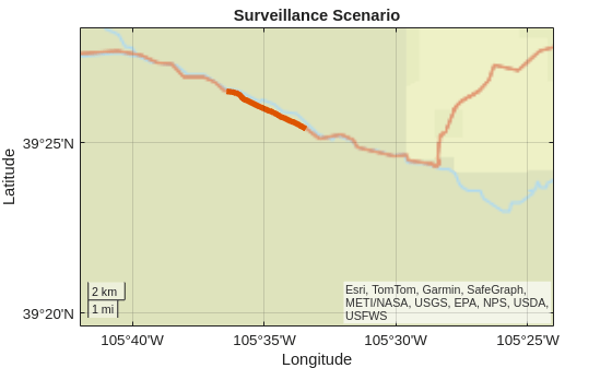

The satellite basemap shows that this portion of the road lies in a mountainous area.

geobasemap satellite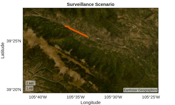

Create a radarScenario and use digital terrain elevation data (DTED) to define this mountainous land surface. Add a LandSurface to the radarScenario with a mountainous surface reflectivity.

scenario = radarScenario(IsEarthCentered=true);
refl = surfaceReflectivityLand(LandType="Mountains");
srf = landSurface(scenario,Terrain="n39_w106_3arc_v2.dt1", ...
    RadarReflectivity=refl);

Use the landSurface height map to assign heights to the road waypoints.

hts = height(scenario.SurfaceManager,[roadLats; roadLons]);
roadLLA = [roadLats; roadLons; hts];

Use helperAddCarsToRoad to add 10 cars along the road. This will add them to the scenario and plot them in the current figure.

helperAddCarsToRoad(scenario,roadLLA)

Define the Radar

Use helperConstantVelocityGeoWaypoints to generate waypoints for a radar platform flying west at 180 knots.

rdrLLA = [39.36 -105.47 7e3]; % [deg deg m]
rdrHeading = 270; % deg, West
rdrSpeed = 180;   % Speed in knots
rdrDur = 60;      % Duration in seconds
[wpts,toa] = helperConstantVelocityGeoWaypoints(rdrLLA,rdrHeading,rdrSpeed,rdrDur);

Add a radar platform to the scenario that uses a geoTrajectory to traverse these waypoints.

rdrPlat = platform(scenario,Trajectory= ...
    geoTrajectory(wpts,toa,ReferenceFrame="ENU"));

Add the radar platform's trajectory and current position to the figure.

geoplot(wpts(:,1),wpts(:,2),SeriesIndex=1)
geoscatter(rdrPlat.Position(1),rdrPlat.Position(2),50,"filled",SeriesIndex=1,DisplayName="Radar")

Mount the radar to the platform looking towards the road over the right-hand side of the platform.

rdrMntLoc = [0 0 0];

Reference the road waypoints to the radar platform's location.

[e,n,u] = geodetic2enu(roadLLA(1,:),roadLLA(2,:),roadLLA(3,:),rdrLLA(1),rdrLLA(2),rdrLLA(3),wgs84Ellipsoid);
posRoad = [e(:) n(:) u(:)];

Find the azimuth spanned by the road in the radar platform's body frame.

rdrPlatAngs = rdrPlat.Orientation;
axesBdy = rotz(rdrPlatAngs(1))*roty(rdrPlatAngs(2))*rotx(rdrPlatAngs(3));

[rgsRoad,angsRoad] = rangeangle(posRoad',rdrMntLoc',axesBdy);
az = angsRoad(1,:);
azSpanRoad = wrapTo180(max(az)-min(az));

Center the radar's antenna pattern on the road.

azRoad = min(az)+azSpanRoad/2;
rdrMntAngs = [azRoad 0 0];

Define a waveform with a maximum unambiguous range large enough to survey the area of interest from the radar platform.

disp(max(rgsRoad)/1e3)

   15.5777

Choose a maximum range of 20 km. This will ensure that the farthest point on the road falls inside of the waveform's unambiguous range.

maxRg = 20e3;

Compute PRF based on max unambiguous range.

prf = 1/range2time(maxRg)

prf = 
7.4948e+03

Use a range resolution of 30 meters to resolve vehicles along the road.

rgRes = 30;

Compute waveform's bandwidth based on the range resolution.

bw = rangeres2bw(rgRes);

Set the sample rate to match the waveform's bandwidth.

Fs = bw;

Ensure that the ratio of the sample rate and PRF is an integer.

prf = Fs/ceil(Fs/prf);

Choose an operating frequency for the radar that provides a maximum unambiguous speed to support vehicle speeds up to 90 miles per hour on the road.

maxSpd = 90;

Choose operating frequency to satisfy maximum unambiguous Doppler requirement.

mps2mph = unitsratio("sm","m")*3600;
lambda = 4*maxSpd/prf/mps2mph;
freq = wavelen2freq(lambda)

freq = 
1.3955e+10

Using 32 pulses enables the radar to resolve radial target speeds to approximately 6 miles per hour, which will further help resolve vehicles along the road.

numPulses = 32;
rrRes = dop2speed(prf/numPulses,lambda)/2;
disp(rrRes*mps2mph)

    5.6250

Use phased.LinearFMWaveform to model the radar waveform.

wfm = phased.LinearFMWaveform(PRF=prf,SweepBandwidth=bw,SampleRate=Fs, ...
    DurationSpecification="Duty cycle",DutyCycle=0.1)

wfm = 
  phased.LinearFMWaveform with properties:

                SampleRate: 4.9965e+06
     DurationSpecification: 'Duty cycle'
                 DutyCycle: 0.1000
                       PRF: 7.4911e+03
     PRFSelectionInputPort: false
            SweepBandwidth: 4.9965e+06
            SweepDirection: 'Up'
             SweepInterval: 'Positive'
                  Envelope: 'Rectangular'
     FrequencyOffsetSource: 'Property'
           FrequencyOffset: 0
              OutputFormat: 'Pulses'
                 NumPulses: 1
             PRFOutputPort: false
    CoefficientsOutputPort: false

While it is possible to model the signals at the output of a monostatic radar's receiver using radarTransceiver, using bistaticTransmitter and a bistaticReceiver to model the two halves of the radar enables you to:

• Simulate clutter signal returns in parallel to speed up simulation

• Include interference in the simulated radar signals

A monostatic radar is a special configuration of the more general bistatic radar, where the transmit and receive antennas are co-located. Create a bistaticTransmitter using the waveform you just defined to model the transmit half of the monostatic radar.

rdrTx = bistaticTransmitter(Waveform=wfm)

rdrTx = 
  bistaticTransmitter with properties:

           Waveform: [1×1 phased.LinearFMWaveform]
        Transmitter: [1×1 phased.Transmitter]
    TransmitAntenna: [1×1 phased.Radiator]
     IsTransmitting: 0
        InitialTime: 0
     SimulationTime: 0

The area of interest along the road spans approximately 6 degrees for the radar platform's trajectory.

disp(azSpanRoad)

    5.7021

The lowest elevation angle along the road is approximately -24 degrees.

disp(min(angsRoad(2,:)))

  -23.7412

Use phased.CosineAntennaElement to define a transmit antenna with a 3 dB azimuth beamwidth of 6 degrees and an elevation beamwidth of 50 degrees to ensure that the entire area of interest is illuminated by the radar.

fov = [6 50]; % [azimuth elevation] degrees
p = log(1/2)./(2*log(cosd(fov/2)));
ant = phased.CosineAntennaElement('CosinePower',p(:)');
figBW = figure;
beamwidth(ant,freq,Cut="Azimuth");

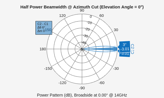
azFOV = beamwidth(ant,freq,Cut="Azimuth")

azFOV = 
6

elFOV = beamwidth(ant,freq,Cut="Elevation")

elFOV = 
49.9200

fov = [azFOV elFOV];

Use this transmit antenna on the bistaticTransmitter.

rdrTx.TransmitAntenna.Sensor = ant;
rdrTx.TransmitAntenna.OperatingFrequency = freq;

Now define the bistaticReceiver for the receive half of the monostatic radar. Define the receive window duration to match the coherent processing interval (CPI) of the waveform used by the transmitter.

cpiDuration = numPulses/prf;
rdrRx = bistaticReceiver(WindowDuration=cpiDuration,SampleRate=Fs);

Set the sample rate used by the receiver.

rdrRx.Receiver.SampleRate = Fs;

Set the MaxCollectDurationSource property to "Property" to set the collect buffer to a fixed size. This enables the clutter returns to be processed in parallel inside of a parfor-loop. Set the duration of the collect buffer to a value larger than the CPI duration. Typically, this value should be set to be several pulse repetition intervals (PRIs) longer than the CPI duration to ensure any signal returns from targets that are ambiguous in range are collected by the buffer.

rdrRx.MaxCollectDurationSource="Property";
rdrRx.MaxCollectDuration=(numPulses+4)/prf;

Create a uniform linear array (ULA) with a 3 dB azimuth beamwidth of at most 2 degrees. This will enable the radar to accurately estimate the azimuth of the vehicles detected along the road.

azRes = 2;

Compute the number of elements in the array based on the azimuth resolution requirement.

d = beamwidth2ap(azRes,lambda,0.8859);
numRxAnt = ceil(2*d./lambda)

numRxAnt = 
51

arr = phased.ULA(numRxAnt,ElementSpacing=lambda/2,Element=ant);

Show that the azimuth resolution requirement is met.

figure(figBW)
beamwidth(arr,freq,Cut="Azimuth");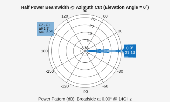

azRes = beamwidth(arr,freq,Cut="Azimuth")

azRes = 
1.9000

Attach the ULA to the bistaticReceiver.

rdrRx.ReceiveAntenna.Sensor = arr;
rdrRx.ReceiveAntenna.OperatingFrequency = freq;

Recall that the area of interest along the road spans around 6 degrees of azimuth. Place multiple beams along the road to cover the entire area of interest.

numBeams = ceil(azSpanRoad/azRes);

For convenience, require that an odd number of beams is used. Using an odd number of beams ensures that one beam will always point along the array's boresight.

if rem(numBeams,2)==0
    numBeams = numBeams+1;
end
disp(numBeams)

     5

azBeams = azRes*(1:numBeams);

The beam azimuths span the azimuth angle occupied by the road.

azBeams = azBeams-mean(azBeams)

azBeams = 1×5

   -3.8000   -1.9000         0    1.9000    3.8000

Use the radarDataGenerator with a clutterGenerator to generate the clutter for the scenario. Create a radarDataGenerator with the same mounting, field of view, range limits, and resolution as the monostatic radar previously defined.

rdr = radarDataGenerator(1,"No scanning", ...
    MountingLocation=rdrMntLoc, ...
    MountingAngles=rdrMntAngs, ...
    CenterFrequency=freq, ...
    FieldOfView=fov, ...
    RangeLimits=[0 maxRg], ...
    AzimuthResolution=azRes, ...
    RangeResolution=rgRes, ...
    RangeRateResolution=rrRes, ...
    HasElevation=false, ...
    HasRangeRate=true);

Set the resolution on the clutterGenerator to have approximately 4 samples for each range resolution bin of the radar to ensure a statistically significant sampling of the ground clutter.

cltrGen = clutterGenerator(scenario,rdr,Resolution=rgRes/4,RangeLimit=maxRg);
rdrPlat.Sensors = rdr;

Use the helperPlotReceiveBeams function to add the beams to the scenario plot.

figure(figScene)
hBms = helperPlotReceiveBeams(rdrPlat,rdrMntAngs,rdrMntLoc,azBeams,maxRg);

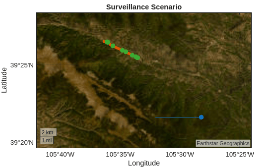
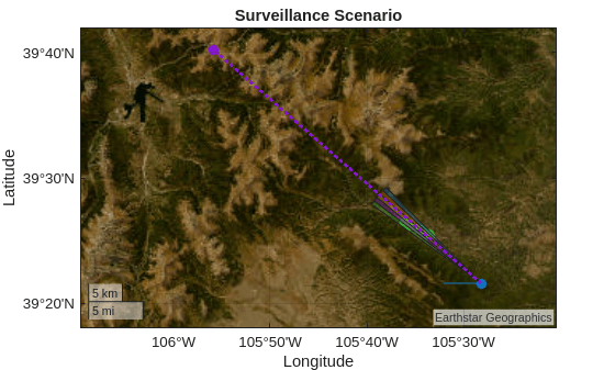
Define the Interfering Emitter

Use bistaticTransmitter to add an antenna tower as an interference source in the scenario. Use a phased.PhaseCodedWaveform to model the signal from the tower. Use a phased.IsotropicAntennaElement to model an antenna tower with a 360-degree coverage area.

twrLat = 39.67;
twrLon = -105.93;
geoscatter(twrLat,twrLon,50,"filled",SeriesIndex=4)
geoplot([rdrLLA(1) twrLat],[rdrLLA(2) twrLon],":",SeriesIndex=4,LineWidth=2,DisplayName="Tower direction")
geolimits([39.3 39.7],[-106.1 -105.4])

twrHt = height(srf,[twrLat;twrLon]);
twrLLA = [twrLat twrLon twrHt];
twrPlat = platform(scenario,Position=twrLLA);

twrTx = bistaticTransmitter();
wfm = phased.PhaseCodedWaveform( ...
    SampleRate=Fs,ChipWidth=1/Fs,PRF=rdrTx.Waveform.PRF);
wfm.NumChips = floor(sqrt(1./(wfm.ChipWidth*wfm.PRF)))^2;
twrTx.Waveform = wfm;

twrTx.TransmitAntenna.Sensor = phased.IsotropicAntennaElement;
twrTx.TransmitAntenna.OperatingFrequency = freq;
disp(twrTx)

  bistaticTransmitter with properties:

           Waveform: [1×1 phased.PhaseCodedWaveform]
        Transmitter: [1×1 phased.Transmitter]
    TransmitAntenna: [1×1 phased.Radiator]
     IsTransmitting: 0
        InitialTime: 0
     SimulationTime: 0

Mount the bistaticTransmitter 10 meters above the ground at the tower's location.

twrMntLoc = [0 0 -10];
twrMntAngs = [0 0 0];

Define a structure array to hold the platform, mounting, next transmit start time, and bistaticTransmitter for the radar transmitter and the antenna tower.

transmitters = [ ...
    struct( ...
    Platform = rdrPlat, ...
    MountingLocation = rdrMntLoc, ...
    MountingAngles = rdrMntAngs, ...
    Transmitter = rdrTx, ...
    NextTime = nextTime(rdrTx)), ...
    struct( ...
    Platform = twrPlat, ...
    MountingLocation = twrMntLoc, ...
    MountingAngles = twrMntAngs, ...
    Transmitter = twrTx, ...
    NextTime = nextTime(twrTx)), ...
    ]

transmitters=1×2 struct array with fields:
    Platform
    MountingLocation
    MountingAngles
    Transmitter
    NextTime

Simulate Radar Signals

Run the simulation to receive signals propagated and collected at the radar receiver from the reflections of the radar pulses from the vehicles along the road and the ground clutter patches as well as the interfering signals from the nearby towers. Stop the simulation once one CPI of data has been received.

isCPIDone = false;
rdrPlsCnt = 0;
hCltr = gobjects(0);
isRunning = advance(scenario);
while isRunning && ~isCPIDone
    simTime = scenario.SimulationTime;    

Propagate and collect signals from each of the transmitters at the radar's receiver.

    for iTx = 1:numel(transmitters)
        thisTx = transmitters(iTx);

Use helperScenarioTruth to get the current pose of transmitter and the target poses. All the other platforms in the scenario other than the current transmit platform are treated as targets.

        [txPose,tgtPoses] = helperScenarioTruth(scenario,thisTx.Platform);
        if thisTx.Platform==rdrPlat

Use freeSpacePath to compute the monostatic propagation paths from the radar's transmitter to the radar's receiver.

            propPaths = freeSpacePath(freq,txPose,tgtPoses, ...
                MountingLocation=thisTx.MountingLocation,MountingAngles=thisTx.MountingAngles);

            rdrPlsCnt = rdrPlsCnt+1;
        else

Use bistaticFreeSpacePath to compute the line-of-sight propagation paths for the interference signal from the antenna tower to the radar's receiver.

            rdrPose = tgtPoses([tgtPoses.PlatformID]==rdrPlat.PlatformID);
            propPaths = bistaticFreeSpacePath(freq,txPose,rdrPose, ...
                TransmitterMountingLocation=thisTx.MountingLocation,TransmitterMountingAngles=thisTx.MountingAngles, ...
                ReceiverMountingLocation=rdrMntLoc,ReceiverMountingAngles=rdrMntAngs);
        end    

Use transmit to generate the signal radiated along each of the propagation paths from the bistaticTransmitter.

        [txSigs,txInfo] = transmit(thisTx.Transmitter,propPaths,simTime);

Allocate a new collection buffer at the start of each CPI.

        if rdrPlsCnt==1 && iTx==1
            [propSigs,propInfo] = collect(rdrRx,simTime);
        end

Collect and coherently combine the signals propagated from each transmitter to the radar's receiver.

        propSigs = propSigs + collect(rdrRx,txSigs,txInfo,propPaths);

Use the clutterGenerator to compute the propagation paths for the clutter patches that lie inside of the radar's transmit beam.

        if thisTx.Platform==rdrPlat
            cltrPaths = clutterTargets(cltrGen);

Use transmit to generate the signals radiated along each clutter path by the radar's bistaticTransmitter.

            [txSigs,txInfo] = transmit(thisTx.Transmitter,cltrPaths,simTime);

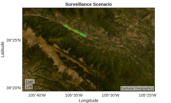
            if rdrPlsCnt==1
                % Update clutter patches on the map
                cdata = clutterRegionData(cltrGen);
                [cltrLat,cltrLon] = deal(cdata.PatchCenters(1,1:1000:end),cdata.PatchCenters(2,1:1000:end));
                if isempty(hCltr) || ~ishghandle(hCltr)
                    
                    hCltr = geoplot(cltrLat,cltrLon,".",LineStyle="none",SeriesIndex=1,MarkerSize=10);
                    geolimits([39.3 39.5],[-105.7 -105.4])
                else
                    set(hCltr,LatitudeData=cltrLat,LongitudeData=cltrLon)
                end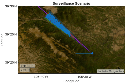

                % Show the number of clutter paths
                disp(numel(cltrPaths));
            end

      301949

Over 300,000 clutter paths are generated for the radar's transmit beam. Processing all these paths at once would require a lot of memory. Use helperWorkerClutterBatches to split the radiated signals and the propagation paths for the clutter into batches to reduce the memory requirements for this simulation. Use a parfor-loop to process these batches in parallel to speed up the simulation. Process no more than 4,000 paths on each worker in each batch.

            [txSigs,cltrPaths] = helperWorkerClutterBatches(txSigs,cltrPaths,4000);

Use a parfor-loop to collect and coherently combine the signals returns from the clutter for each batch of clutter paths.

            for iBatch = 1:numel(txSigs)
                [sigBatches,pathBatches] = deal(txSigs{iBatch},cltrPaths{iBatch});
                parfor iWorker = 1:numel(sigBatches)
                    propSigs = propSigs + collect(rdrRx,sigBatches{iWorker},txInfo,pathBatches{iWorker});
                end
            end
        end

Use nextTime to compute the start time for this transmitter's next transmission.

        transmitters(iTx).NextTime = nextTime(thisTx.Transmitter);
    end

Use nextTime to compute the start time of the next receive window. Continue advancing the simulation collecting transmissions from all the transmitters until the start time of the next receive window has been reached.

    nextRdrRx = nextTime(rdrRx);
    nextTx = [transmitters.NextTime];
    isCPIDone = all(nextRdrRx<=nextTx);
    if isCPIDone

When all the transmissions for this CPI have been propagated and collected, it is time to receive the signals. Advance the scenario forward to the end of the receive window and use receive to receive the collected signals.

        tStep = nextRdrRx - scenario.SimulationTime;
        if tStep>0
            scenario.UpdateRate = 1/tStep;
            isRunning = advance(scenario);
        end
        % Update the bistaticReceiver to the current simulation time
        collect(rdrRx,scenario.SimulationTime);

        % Receive the collected signals
        [rxSig,rxInfo] = receive(rdrRx,propSigs,propInfo);
    end

Step the simulation forward to the next transmission time and continue propagating and collecting signals until the end of the CPI has been reached.

    tStep = min(nextTx) - scenario.SimulationTime;
    if tStep>0
        scenario.UpdateRate = 1/tStep;
        isRunning = advance(scenario);
    end
end

Process Simulated Radar Signals

Reshape the received radar signals to form a radar datacube that has dimensions equal to the number of fast-time samples by number of spatial channels by number of slow-time samples.

numFT = Fs/prf;    % Number of fast-time samples
numCh = numRxAnt;  % Number of spatial channels
numST = numPulses; % Number of slow-time samples

xCube = permute(reshape(rxSig,numFT,numST,numCh),[1 3 2]);
disp(size(xCube))

   667    51    32

Compute the noise floor of the simulated radar data using the properties on the radar's receiver.

kb = physconst("Boltzmann");
nFctr = db2pow(rdrRx.Receiver.NoiseFigure);
nPwrdB = pow2db(kb*(nFctr-1)*rdrRx.Receiver.ReferenceTemperature*rdrRx.Receiver.SampleRate) + rdrRx.Receiver.Gain

nPwrdB = 
-117.0091

Use phased.RangeDopplerResponse to apply range and Doppler processing to the radar datacube.

mfcoeff = getMatchedFilter(rdrTx.Waveform);
procRgDp = phased.RangeDopplerResponse( ...
    DopplerOutput="Range rate", ...
    DopplerWindow="Hamming", ...
    OperatingFrequency=rdrRx.ReceiveAntenna.OperatingFrequency, ...
    SampleRate=rdrRx.Receiver.SampleRate);
procRgDp.DopplerWindow = "None";

[xRgDp,binsRg,binsRr] = procRgDp(xCube,mfcoeff);

Compute the range and Doppler processing gains.

Grg = pow2db(mfcoeff'*mfcoeff)

Grg = 
18.2607

Gdp = pow2db(numST)

Gdp = 
15.0515

Compute the range rate of the ground clutter in the antenna's boresight direction.

rdrMntAxes = rotz(rdrMntAngs(1))*roty(rdrMntAngs(2))*rotx(rdrMntAngs(3));
boresightDir = rdrMntAxes(:,1);

Find locations on the ground along the antenna's boresight direction.

rgGnd = 10e3:1e3:maxRg-time2range(rdrTx.Waveform.DutyCycle/rdrTx.Waveform.PRF);
posGnd = rgGnd.*boresightDir + rdrMntLoc(:);

Compute the ground locations in the scenario's Earth-Centered, Earth-Fixed (ECEF) coordinate frame.

rdrPose = helperScenarioTruth(scenario,rdrPlat);
rdrPlatAxes = rotmat(rdrPose.Orientation,"frame")';

posGnd = rdrPlatAxes*posGnd + rdrPose.Position(:);
[ltGnd,lnGnd] = ecef2geodetic(wgs84Ellipsoid,posGnd(1,:),posGnd(2,:),posGnd(3,:));
htGnd = height(srf,[ltGnd;lnGnd])

htGnd = 1×8
103 ×

    2.5780    2.5550    2.5225    2.4951    2.5541    2.5960    2.6963    2.7600

[x,y,z] = geodetic2ecef(wgs84Ellipsoid,ltGnd,lnGnd,htGnd);
posGnd = [x;y;z];

Compute the velocity of the ground relative to the radar platform's motion.

velGnd = -rdrPose.Velocity(:); % In ECEF

The range rate of the ground clutter in the direction of the antenna's boresight is the dot-product of the velocity of the ground relative to the platform's motion with the direction to the ground locations.

dirGnd = posGnd-rdrPose.Position(:);
rgGnd = sqrt(sum(dirGnd.^2,1));
dirGnd = dirGnd./rgGnd;
rrGnd = velGnd'*dirGnd % dot-product

rrGnd = 1×8

  -64.4521  -65.3398  -66.0267  -66.5886  -67.1686  -67.6204  -68.0565  -68.3813

Wrap the computed range rate based on the maximum range rate supported by the radar's waveform.

rrMax = dop2speed(prf/2,lambda)/2

rrMax = 
40.2337

rrGnd = wrapToPi(rrGnd*pi/rrMax)*rrMax/pi

rrGnd = 1×8

   16.0153   15.1275   14.4407   13.8788   13.2988   12.8469   12.4108   12.0860

Compute the range rate of the antenna tower's signal observed by the radar.

[x,y,z] = geodetic2ecef(wgs84Ellipsoid,twrPlat.Position(1),twrPlat.Position(2),twrPlat.Position(3));
twrPos = [x;y;z];
twrDir = twrPos-rdrPose.Position(:);
twrDir = twrDir/norm(twrDir)

twrDir = 3×1

   -0.5990
    0.6516
    0.4655

The tower's apparent velocity relative to the radar platform is the same as the velocity of the ground.

twrVel = -rdrPose.Velocity(:);

Because the range rate computed by a monostatic radar assumes the received signal traversed a two-way path, division by two is necessary to account for the fact that the tower's signal only traverses a one-way path to the radar.

rrTwr = dot(twrVel,twrDir)/2;
rrTwr = wrapToPi(rrTwr*pi/rrMax)*rrMax/pi

rrTwr = 
-34.8011

Use the helperBeamform function to compute the receive beams and beamforming gain.

sv = steervec(getElementPosition(rdrRx.ReceiveAntenna.Sensor)/lambda,azBeams);
[xBm,Gbf] = helperBeamform(xRgDp,sv);
disp(size(xBm))

   667     5    32

disp(Gbf)

   17.0757   17.0757   17.0757   17.0757   17.0757

function [xBm,Gbf] = helperBeamform(xCube,w)
% Returns a beamformed datacube using the provided steering weights
[numFT,numCh,numST] = size(xCube);
numBeams = size(w,2);
xBm = permute(xCube,[2 1 3]); % Number of channels by number of range bins by number of Doppler bins
xBm = reshape(xBm,numCh,numFT*numST);
xBm = w'*xBm;
xBm = reshape(xBm,numBeams,numFT,numST);
xBm = permute(xBm,[2 1 3]);   % Number of range bins by number of beams by number of Doppler bins

if nargout>1
    Gbf = pow2db(sum(abs(w).^2,1));
end
end

Compute the noise floor after radar signal processing gains.

ndB = nPwrdB + Grg + Gdp + Gbf

ndB = 1×5

  -66.6212  -66.6212  -66.6212  -66.6212  -66.6212

Select the center receive beam pointed along the antenna's boresight direction.

iBeam = ceil(numBeams/2);
disp(azBeams(iBeam))

     0

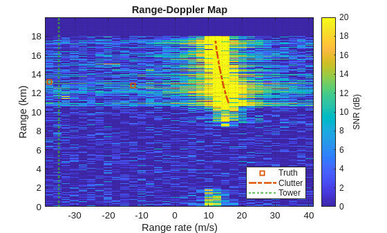
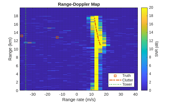
Use the helperRangeDopplerMap function to plot the range-Doppler map for the range, Doppler, and beamform processed radar datacube for the center receive beam.

helperRangeDopplerMap(iBeam,xBm,ndB,binsRg,azBeams,binsRr,rgGnd,rrGnd,rdrPlat,rdrMntAngs,rdrMntLoc)
clim([0 65])

Add the expected range rate of the antenna tower's signal to the range-Doppler map.

xline(rrTwr,":",LineWidth=2,SeriesIndex=5,DisplayName="Tower")

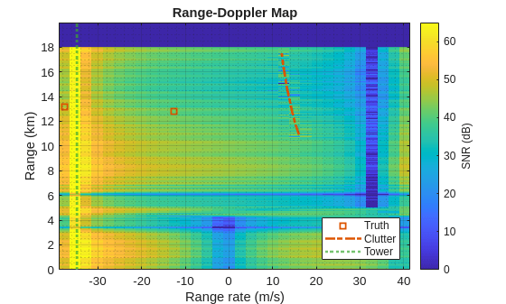
The antenna tower's signal and the clutter returns are visible in the radar data on the left and right sides of the range-Doppler map respectively.

Use the helperPlotRangeAngle function to overlay the received signal power in the radar datacube on the geographic axes. Compute the angle response across the transmit antenna's field of view. helperPlotRangeAngle selects the maximum power across the Doppler bins for each range-angle cell to reduce the data to two dimensions for visualization purposes.

azScan = fov(1)*linspace(-1,1,101);
svScan = steervec(getElementPosition(rdrRx.ReceiveAntenna.Sensor)/lambda,azScan);

figure(figScene)
ndB = nPwrdB + Grg + Gdp;
hRgAz = helperPlotRangeAngle(svScan,xRgDp,binsRg,azScan,ndB,rdrPose,rdrMntAngs,rdrMntLoc);
clim([0 75])
ylabel(colorbar,"SNR (dB)")
set(hBms,Visible="off")
set(hCltr,Visible="off")

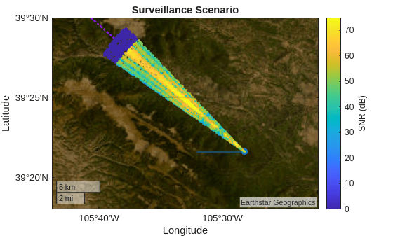
The range-angle response is dominated by the antenna tower's signal received at the radar.

Use sensorcov and mvdrweights to place a null in the direction of the antenna tower. First, compute the angle of the antenna tower relative to the radar antenna's mounted location and orientation.

[x,y,z] = geodetic2ecef(wgs84Ellipsoid,twrPlat.Position(1),twrPlat.Position(2),twrPlat.Position(3));
twrPos = [x;y;z];
twrPos = rdrPlatAxes'*(twrPos-rdrPose.Position(:));
[~,twrAng] = rangeangle(twrPos,rdrMntLoc(:),rdrMntAxes)

twrAng = 2×1

   -0.7021
   -3.8301

Now compute a sensor spatial covariance matrix for a signal arriving from the direction of the tower with a noise floor matching the noise floor at the output of the range and Doppler processor.

ndB = nPwrdB + Grg + Gdp;
Sn = sensorcov(getElementPosition(rdrRx.ReceiveAntenna.Sensor)/lambda,twrAng,db2pow(ndB));

Use mvdrweights to show the range-angle response with a null placed in the direction of the antenna tower.

swScan = mvdrweights(getElementPosition(rdrRx.ReceiveAntenna.Sensor)/lambda,azScan,Sn);

figure(figScene)
delete(hRgAz)
hRgAz = helperPlotRangeAngle(swScan,xRgDp,binsRg,azScan,ndB,rdrPose,rdrMntAngs,rdrMntLoc);
clim([0 75])
ylabel(colorbar,"SNR (dB)")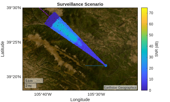

The spatial null suppresses the antenna tower's signal.

Now, compute the receive beams using the same spatial covariance matrix and the beam azimuths computed earlier.

sw = mvdrweights(getElementPosition(rdrRx.ReceiveAntenna.Sensor)/lambda,azBeams,Sn);

Normalize the receive beam weights.

sw = sw./sqrt(sum(abs(sw).^2,1));

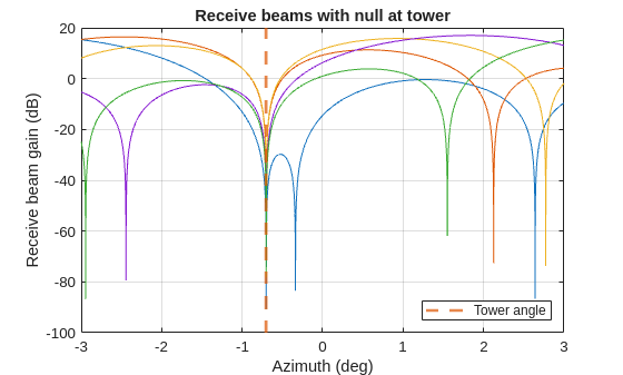
Show the beam patterns for the minimum variance, distortionless response (MVDR) receive beam weights.

figure
azScan = fov(1)/2*linspace(-1,1,1e4);
svScan = steervec(getElementPosition(rdrRx.ReceiveAntenna.Sensor)/lambda,azScan);
plot(azScan,mag2db(abs(svScan'*sw)))
p = xline(twrAng(1),"--",SeriesIndex=2,LineWidth=2,DisplayName="Tower angle");
xlabel("Azimuth (deg)");
ylabel("Receive beam gain (dB)")
title("Receive beams with null at tower")
grid on
legend(p,Location="southeast");

[xBm,Gbf] = helperBeamform(xRgDp,sw);
disp(Gbf)

     0     0     0     0     0

Compute the noise floor after radar signal processing gains.

ndB = nPwrdB + Grg + Gdp + Gbf;

Plot the range-Doppler response along the receive array's boresight direction with a null in the direction of the antenna tower.

helperRangeDopplerMap(iBeam,xBm,ndB,binsRg,azBeams,binsRr,rgGnd,rrGnd,rdrPlat,rdrMntAngs,rdrMntLoc)
xline(rrTwr,":",LineWidth=2,SeriesIndex=5,DisplayName="Tower")

You can see that the spatial null mitigated the antenna tower signal in the range-Doppler response in the boresight beam direction.

Zoom in along the range axis to see the targets inside this receive beam.

[tgtAngs,tgtRg] = helperRadarTruth(rdrPlat,rdrMntAngs,rdrMntLoc,maxRg);
inBeam = find(abs(wrapTo180(tgtAngs(1,:)-azBeams(iBeam)))<=azRes/2);
rgSpan = max(tgtRg(inBeam))-min(tgtRg(inBeam));
rgLim = max(rgSpan,1e3)/2*[-1 1]+min(tgtRg(inBeam))+rgSpan/2;
ylim(rgLim/1e3)

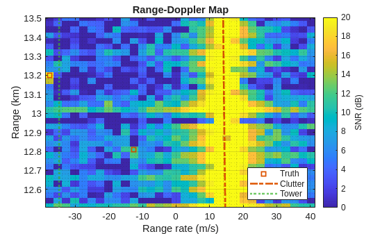
The cars along the road are now visible in the range-Doppler map, but there is still strong clutter interference that will generate undesired target detections and mask some of the targets without additional processing.

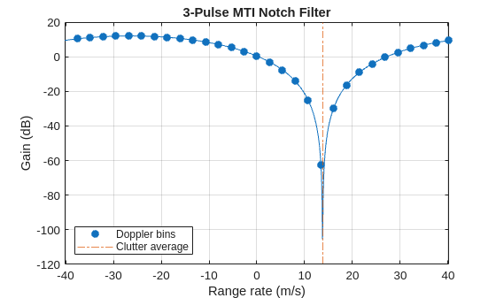
Use a 3-pulse moving target indicator (MTI) notch filter to place a Doppler null on the ground clutter returns. Define the MTI filter using a binomial taper.

wMTI = [1 2 1];

Use dopsteeringvec to place the filter's notch at the average expected Doppler of the ground clutter.

fd = -2*speed2dop(mean(rrGnd),lambda);
fMax = prf/2;
fd = wrapTo180((fd+prf/2)*180/fMax)*fMax/180;
K = numel(wMTI);
M = numST-K+1;

vt = dopsteeringvec(fd,K,prf);
wt = wMTI(:).*vt;

Show that the Doppler response of the 3-pulse MTI notch filter places a null at the expected Doppler of the ground clutter.

dp = linspace(-0.5,0.5,1e3);
dft = dopsteeringvec(dp,K);
Hmti = mag2db(abs(dft'*wt));
rr = -dop2speed(dp*prf,lambda)/2;

figure
plot(rr,Hmti)

rr = fliplr(((1:M)/M-0.5)*2*rrMax);
dp = speed2dop(-2*rr,lambda);
dft = dopsteeringvec(dp,K,prf);
Gmti = mag2db(abs(dft'*wt))';

hold on
p1 = plot(rr,Gmti,"o",SeriesIndex=1,DisplayName="Doppler bins");
p1.MarkerFaceColor = p1.Color;
p2 = xline(mean(rrGnd),"-.",SeriesIndex=2,DisplayName="Clutter average");

xlabel("Range rate (m/s)");
ylabel("Gain (dB)");
title("3-Pulse MTI Notch Filter");
grid("on")

xlim(max(rr)*[-1 1])
legend([p1 p2],Location="southwest")

Apply the MTI notch filter to the radar datacube.

xMTI = zeros(numFT,numCh,M);
for k = 1:K
    xMTI = xMTI + conj(wt(k))*xCube(:,:,(1:M)+(k-1));
end

Use phased.RangeDopplerResponse to apply range and Doppler processing to the radar datacube after the MTI filtering has been applied.

procRgDp = phased.RangeDopplerResponse( ...
    DopplerWindow="Hamming", ...
    DopplerOutput="Range rate", ...
    OperatingFrequency=rdrRx.ReceiveAntenna.OperatingFrequency, ...
    SampleRate=rdrRx.Receiver.SampleRate);
[xRgDp,binsRg,binsRr] = procRgDp(xMTI,mfcoeff);

Compute the range and Doppler processing gains.

Grg = pow2db(mfcoeff'*mfcoeff)

Grg = 
18.2607

Gdp = pow2db(M)

Gdp = 
14.7712

Apply beamforming with a null in the direction of the antenna tower.

[xBm,Gbf] = helperBeamform(xRgDp,sw);

Compute the noise floor after all of the radar signal processing.

Gmti = reshape(Gmti,1,1,M);
ndB = nPwrdB + Gmti + Grg + Gdp + Gbf;
disp(size(ndB))

     1     5    30

Plot the range-Doppler response along the receive array's boresight direction.

iBeam = ceil(numBeams/2);
helperRangeDopplerMap(iBeam,xBm,ndB,binsRg,azBeams,binsRr,rgGnd,rrGnd,rdrPlat,rdrMntAngs,rdrMntLoc)
xline(rrTwr,":",LineWidth=2,SeriesIndex=5,DisplayName="Tower")

The MTI pulse canceller suppresses the ground clutter in the radar datacube.

Zoom in along the range axis to see the targets inside this receive beam.

[tgtAngs,tgtRg] = helperRadarTruth(rdrPlat,rdrMntAngs,rdrMntLoc,maxRg);
inBeam = find(abs(wrapTo180(tgtAngs(1,:)-azBeams(iBeam)))<=azRes/2);
rgSpan = max(tgtRg(inBeam))-min(tgtRg(inBeam));
rgLim = max(rgSpan,1e3)/2*[-1 1]+min(tgtRg(inBeam))+rgSpan/2;
ylim(rgLim/1e3)

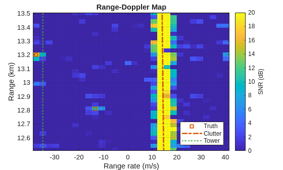
The cars along the road now stand out much more clearly in the range-Doppler map, because most of the clutter interference was removed by the MTI notch filter.

Use phased.CFARDetector2D to estimate the remaining interference and clutter background power level and to identify the target returns in the processed datacube. Use the estimated background power level to compute the signal to interference and noise ratio (SINR).

ndB = nPwrdB + Gmti + Grg + Gdp + Gbf;
xSNRdB = mag2db(abs(xBm))-ndB;

cfar = phased.CFARDetector2D( ...
    GuardBandSize=[1 1], ...
    TrainingBandSize=[20 1], ...
    ProbabilityFalseAlarm=1e-6, ...
    NoisePowerOutputPort=true);

Use the helperCFAR2D function to estimate the background power level and identify the target locations.

[dets,bgdB] = helperCFAR2D(cfar,xSNRdB);

Define a minimum detectable target velocity corresponding to 1.5 range rate bins from the clutter ridge location. Ignore any detections inside of this region.

minDetVel = 1.5*rrRes;
iRrGnd = find(abs(binsRr-mean(rrGnd))<=minDetVel);
isGd = ~ismember(dets(:,3),iRrGnd);
dets = dets(isGd,:);

figure
plot(binsRr,squeeze(pow2db(mean(db2pow(bgdB(binsRg>2e3&binsRg<16e3,iBeam,:)),1))));
p1 = xline(mean(rrGnd),"-.",LineWidth=2,SeriesIndex=2,DisplayName="Clutter");
p2 = xline(mean(rrGnd)+minDetVel*[-1 1],"--",LineWidth=2,SeriesIndex=2,DisplayName="Minimum detectable velocity");
xlabel("Range rate (m/s)")
ylabel("Background power (dB)")
title("CFAR background estimate")
grid on
legend([p1 p2(1)],Location="northwest");

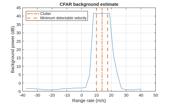
As expected, the background power level is near 0 everywhere except for near the clutter ridge where some of the clutter persists despite the MTI notch filter.

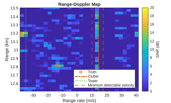
xSINRdB = xSNRdB-bgdB;

Show the range-Doppler map using the SINR estimated using the constant false alarm rate (CFAR) detector.

iBeam = ceil(numBeams/2);
helperRangeDopplerMap(iBeam,db2mag(xSINRdB),0*ndB,binsRg,azBeams,binsRr,rgGnd,rrGnd,rdrPlat,rdrMntAngs,rdrMntLoc)
xline(rrTwr,":",LineWidth=2,SeriesIndex=5,DisplayName="Tower")
xline(mean(rrGnd)+1.5*rrRes*[-1 1],"--",LineWidth=2,SeriesIndex=2,DisplayName="Minimum detectable velocity");
ylabel(colorbar,"SINR (dB)")
ylim(rgLim/1e3)
p = legend;
p.String = p.String(1:end-1);

Plot the CFAR detections and overlay the true target locations in range and range rate.

rgBinDets = binsRg(dets(:,1));
rrBinDets = binsRr(dets(:,3));

[~,tgtRg,tgtRr] = helperRadarTruth(rdrPlat,rdrMntAngs,rdrMntLoc,maxRg);
tgtRr = wrapTo180(tgtRr*180/rrMax)*rrMax/180;

figDets = figure;
plot(rrBinDets,rgBinDets/1e3,"o",tgtRr,tgtRg/1e3,"*")
xlabel("Range rate (m/s)")
ylabel("Range (km)")
title("CFAR detections and true targets")
grid on
legend("CFAR detections","True targets",Location="eastoutside")

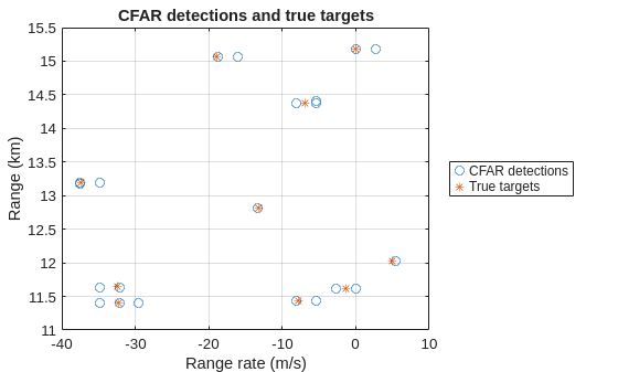
Multiple detections are generated from the targets. This is because the same target can appear in adjacent range and range rate bins as well as in adjacent beams.

Use clusterDBSCAN to group the detections coming from the same target. Perform the clustering using the range and range rate bins for the CFAR detections since these provide the highest resolution for the radar. The cross-range resolution in meters for the azimuth beam is too large at the target range to help discern detections from the different vehicles along the road.

epsilon = 5;
cluster = clusterDBSCAN(Epsilon=epsilon,MinNumPoints=2, ...
    EnableDisambiguation=true,AmbiguousDimension=2);
ambLims = [-rrMax rrMax]; % range rate wraps, so this dimension is ambiguous
[~,ids] = cluster([rgBinDets rrBinDets],ambLims);

Find the number of unique detection clusters.

uIDs = unique(ids);
numDets = numel(uIDs)

numDets = 
12

figure(figDets)
hold on
for iDet = 1:numDets
    iFnd = ids==uIDs(iDet);
    plot(rrBinDets(iFnd),rgBinDets(iFnd)/1e3,".-",SeriesIndex=iDet,MarkerSize=10,DisplayName=sprintf("Cluster %i",iDet));
end

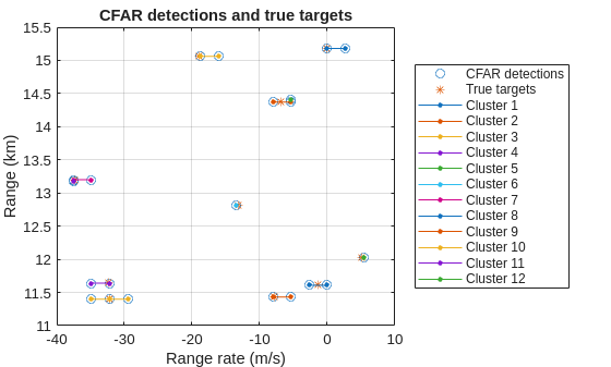
You can see that the clustering algorithm grouped multiple detections so that most clusters correspond to actual car targets.

Use refinepeaks to estimate the range and azimuth for each detection cluster.

estRgs = NaN(1,numDets);
estAzs = NaN(1,numDets);
estSINRdB = NaN(1,numDets);
for iDet = 1:numDets
    % Find the detections associated with this cluster.
    iFnd = find(ids==uIDs(iDet));
    iDets = dets(iFnd,:);
    ind = sub2ind(size(xSINRdB),iDets(:,1),iDets(:,2),iDets(:,3));

    % Find the local maximum in the cluster
    [pk0,iMax] = max(xSINRdB(ind));
    ind = iDets(iMax,:);

    % Estimate the range of the cluster
    y = db2mag(xSINRdB(:,ind(2),ind(3)));
    iRg = ind(1);
    iPk = iRg+(-1:1);
    iPk = iPk(iPk>0 & iPk<=size(xSINRdB,1));
    [~,iMax] = max(y(iPk));
    iRg = iPk(iMax);
    [pk1,estRgs(iDet)] = refinepeaks(y,iRg,binsRg);

    % Estimate the azimuth of the cluster
    y = db2mag(xSINRdB(ind(1),:,ind(3)));
    iPk = ind(2)+(-2:2);
    iPk = iPk(iPk>0 & iPk<=numBeams);
    [~,iMax] = max(y(iPk));
    iBeam = iPk(iMax);
    [pk2,estAzs(iDet)] = refinepeaks(y,iBeam,azBeams);

    estSINRdB(iDet) = mag2db(max([db2mag(pk0) pk1 pk2]));
end

Estimate the elevation of detections to be on the road since this radar measures azimuth angle but not elevation angle.

elSpanRoad = wrapTo180(max(angsRoad(2,:))-min(angsRoad(2,:)));
estEls = min(angsRoad(2,:))+elSpanRoad/2;

Show the estimated detection locations in the scenario.

pos = zeros(3,numDets);
[pos(1,:),pos(2,:),pos(3,:)] = sph2cart(deg2rad(estAzs),deg2rad(estEls),estRgs);
pos = rdrMntAxes*pos + rdrMntLoc(:);
pos = rdrPlatAxes*pos + rdrPose.Position(:);
[detLats,detLons] = ecef2geodetic(wgs84Ellipsoid,pos(1,:),pos(2,:),pos(3,:));

figure(figScene)
hRgAz.Visible = "off";
geoscatter(detLats,detLons,70,estSINRdB,"filled",Marker="diamond",MarkerEdgeColor="black",DisplayName="Detections");
legend(findobj(gca().Children,"-not",DisplayName=""))
geolimits([39.35 39.45],[-105.6 -105.5])
clim([0 20])

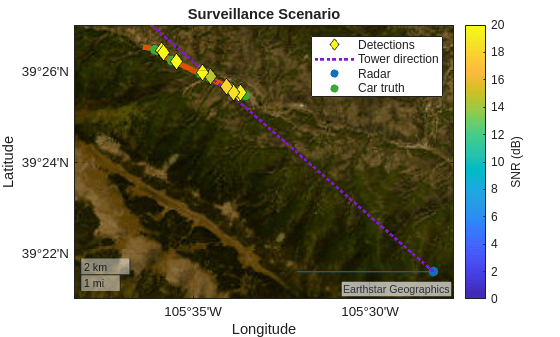
The estimated locations for the detections are located along the road and are likely to be true detections from the cars and not from the interference or clutter. The spatial and temporal filters enabled the cars to be detected in the presence of significant interference and clutter.

Summary

In this example you learned how to use bistaticTransmitter and bistaticReceiver objects to model both halves of a monostatic radar. You also used bistaticTransmitter to model an interference source in the radar's field of view. The bistaticReceiver was used with a parfor-loop to speed up the simulation by processing the propagation of the clutter returns in parallel. Finally, you placed nulls on the interference and clutter signals using spatial and temporal filters respectively, enabling some of the vehicle detections along the road to be recovered.

Helper Functions

function [sigBatches,pathBatches] = helperWorkerClutterBatches(txSigs,propPaths,maxPathsPerWorker)
% Returns batches of transmit signals and corresponding propagation paths
% for batch processing to reduce memory requirements for modeling clutter
% returns. Each batch is limited to a maximum number of propagation paths
% per worker, where the number of workers is defined by the parallel pool.
% The returned batches can be processed using a parfor-loop.

arguments
    txSigs
    propPaths
    maxPathsPerWorker = 1000
end

persistent numWorkers
if isempty(numWorkers)
    pool = gcp;
    numWorkers = pool.NumWorkers;
end

numPaths = numel(propPaths);
maxNumPathsPerWorker = min(ceil(numPaths/numWorkers),maxPathsPerWorker);
numBatches = ceil(numPaths/(maxNumPathsPerWorker*numWorkers));
sigBatches = cell(1,numBatches);
pathBatches = cell(1,numBatches);

ind = 0;
for iBatch = 1:numBatches
    theseSigs = cell(numWorkers,1);
    thesePaths = cell(numWorkers,1);
    for iWorker = 1:numWorkers
        numPathsInBatch = min(maxNumPathsPerWorker,numPaths);

        iPaths = (1:numPathsInBatch)+ind;
        theseSigs{iWorker} = txSigs(:,iPaths);
        thesePaths{iWorker} = propPaths(iPaths);

        ind = iPaths(end);
        numPaths = numPaths-numPathsInBatch;
        if numPaths<1
            break
        end
    end

    % Remove unused batches
    isUsed = ~cellfun(@isempty,theseSigs);
    theseSigs = theseSigs(isUsed);
    thesePaths = thesePaths(isUsed);

    sigBatches{iBatch} = theseSigs;
    pathBatches{iBatch} = thesePaths;
end
end

function helperRangeDopplerMap(iBeam,sig,nPwrdB,binsRg,azBeams,binsRr,rgGnd,rrGnd,rdrPlat,rdrMntAngs,rdrMntLoc)
% Plots a range-Doppler map and with target truth overlayed on top. 

xSNRdB = mag2db(abs(sig))-nPwrdB;
xSNRdB = squeeze(xSNRdB(:,iBeam,:));

ax = axes(figure);
imagesc(ax,binsRr,binsRg/1e3,squeeze(xSNRdB));
xlabel(ax,"Range rate (m/s)"); ylabel(ax,"Range (km)");
title(ax,"Range-Doppler Map");
clim(ax,[0 20]);
ylabel(colorbar(ax),"SNR (dB)");
grid(ax,"on"); grid(ax,"minor");
ax.Layer = "top";
ax.YDir = "normal";
hold(ax,"on");
axis(ax,"tight");
axis(ax,axis(ax));

[tgtAngs,tgtRg,tgtRr] = helperRadarTruth(rdrPlat,rdrMntAngs,rdrMntLoc,max(binsRg));

% Remove targets outside of the selected beam
azRes = diff(azBeams(1:2));
azs = wrapTo180(tgtAngs(1,:)-azBeams(iBeam));
inBeam = abs(azs)<=azRes/2;
tgtRg = tgtRg(inBeam);
tgtRr = tgtRr(inBeam);

% Resolve the target truth to the resolution bins
resRg = diff(binsRg(1:2));
tgtRg = round(tgtRg/resRg)*resRg;

resRr = diff(binsRr(1:2));
tgtRr = round(tgtRr/resRr)*resRr;

% Compute max range rate
maxRr = max(abs(binsRr));

% Wrap to +/- maxRr
tgtRr = wrapTo180(tgtRr*180/maxRr)*maxRr/180;

p1 = plot(ax,tgtRr,tgtRg/1e3,"s",LineWidth=2,SeriesIndex=2,DisplayName="Truth");
p2 = plot(ax,rrGnd,rgGnd/1e3,"-.",LineWidth=2,SeriesIndex=2,DisplayName="Clutter");
legend([p1 p2],Location="southeast");
end

function [tgtAngs,tgtRg,tgtRr] = helperRadarTruth(rdrPlat,rdrMntAngs,rdrMntLoc,maxRg)
% Returns the target truth in the radar's spherical coordinates

tposes = targetPoses(rdrPlat);
tpos = reshape([tposes.Position],3,[]);

rdrMntAxes = rotz(rdrMntAngs(1))*roty(rdrMntAngs(2))*rotx(rdrMntAngs(3));
[tgtRg,tgtAngs] = rangeangle(tpos,rdrMntLoc(:),rdrMntAxes);

tvel = reshape([tposes.Velocity],3,[]);
tgtRr = sum(tvel.*(tpos./tgtRg),1);

% Remove targets outside of the max range
inRg = tgtRg<=maxRg;
tgtAngs = tgtAngs(:,inRg);
tgtRg = tgtRg(inRg);
tgtRr = tgtRr(inRg);
end

function [dets,bgdB] = helperCFAR2D(cfar,xSNRdB)
% Applies the 2D CFAR detector to each beam in the processed datacube.
% Returns an L-by-3 matrix containing the 3D detection indices for the L
% detections found in the data. Returns a datacube with the same size as
% the processed datacube containing the CFAR background estimate in
% decibels.
[numRg,numBeams,numRr] = size(xSNRdB);
bgdB = zeros(numRg,numBeams,numRr);
dets = zeros(0,3);
totBandSz = cfar.TrainingBandSize+cfar.GuardBandSize;

iRgCUT = totBandSz(1)+1:numRg-totBandSz(1);

% Pad the data in Doppler so that it wraps
iDp1 = mod((-(totBandSz(2)-1):0)-1,numRr)+1;
iDp2 = mod(numRr+(1:totBandSz(2))-1,numRr)+1;

iRrCUT = (1:numRr)+totBandSz(2);
[iRr,iRg] = meshgrid(iRrCUT,iRgCUT);
iCUT = [iRg(:) iRr(:)].';
for iBeam = 1:numBeams
    snr = db2pow(squeeze(xSNRdB(:,iBeam,:)));

    % Pad the data in Doppler so that it wraps
    snr = [snr(:,iDp1) snr snr(:,iDp2)]; %#ok<AGROW>
    
    [isDet,intPwr] = cfar(snr,iCUT);
    iDet = iCUT(:,isDet(:));
    numDets = size(iDet,2);
    dets = cat(1,dets,[iDet(1,:);iBeam*ones(1,numDets);iDet(2,:)-totBandSz(2)]');

    ind = sub2ind([numRg numBeams numRr],iCUT(1,:)',iBeam*ones(size(iCUT,2),1),iCUT(2,:)'-totBandSz(2));
    bgdB(ind) = pow2db(intPwr);
end
end

function [rdrPose,tgtPoses] = helperScenarioTruth(scenario,rdrPlat)
% Returns scenario truth pose struct arrays with radar cross section (RCS)
% included for the radar platform and the remaining target platforms. All
% target poses are returned in the scenario frame.

poses = platformPoses(scenario);
profiles = platformProfiles(scenario);
ids = [profiles.PlatformID];
for m = 1:numel(poses)
    iFnd = find(ids==poses(m).PlatformID,1);
    poses(m).Signatures = profiles(iFnd).Signatures;
end

ids = [poses.PlatformID];
isTgt = ids~=rdrPlat.PlatformID;
rdrPose = poses(~isTgt);
tgtPoses = poses(isTgt);
end

function [wpts,toa] = helperConstantVelocityGeoWaypoints(startLLA,heading,speed,dur)
% Returns a platform traveling at a constant speed and bearing.

kts2mps = unitsratio("m","nm")/3600;
speed = speed*kts2mps;

dist = speed*dur;

[latEnd, lonEnd] = reckon(startLLA(1), startLLA(2), dist, heading, wgs84Ellipsoid);
wpts = [startLLA;latEnd lonEnd startLLA(3)];
toa = [0 dur];
end

function helperAddCarsToRoad(scenario,wptsRoad,nvPairs)
% Adds cars distributed randomly along the length of the road defined by
% the waypoints. Car speeds a uniformly distributed between 20 and 80 miles
% per hour and are traveling in both directions along the road with equal
% probability.
arguments
    scenario
    wptsRoad
    nvPairs.NumCars = 10
    nvPairs.MinMaxMPH = [20 80]
    nvPairs.RCSdBsm = 20
end

earth = wgs84Ellipsoid;

% Place cars randomly along the road
[x,y,z] = geodetic2enu(wptsRoad(1,:),wptsRoad(2,:),wptsRoad(3,:),wptsRoad(1,1),wptsRoad(2,1),wptsRoad(3,1),earth);
enu = [x(:) y(:) z(:)];
dist = cumsum([0;sqrt(sum(diff(enu,1,1).^2,2))]);

span = dist(end);
d0 = span*rand(nvPairs.NumCars,1) + (dist(end)-span)/2;

% Assign random speeds to cars
mph2mps = unitsratio("m","sm")/3600;
spdlim = nvPairs.MinMaxMPH*mph2mps;
spds = diff(spdlim)*rand(nvPairs.NumCars,1) + min(spdlim);
dir = rand(size(spds));
spds(dir<0.5) = -spds(dir<0.5);

% Create a platform for each car
carRCS = rcsSignature(Pattern=nvPairs.RCSdBsm);
tStop = scenario.StopTime;
if ~isfinite(tStop)
    tStop = 1;
end
toas = linspace(0,tStop)';
llaStart = NaN(3,nvPairs.NumCars);
for m = 1:nvPairs.NumCars
    % Interpolate points along the road to define the car's trajectory
    ds = spds(m)*toas + d0(m);
    wpts = interp1(dist,enu,ds);
    [lts,lns,hts] = enu2geodetic(wpts(:,1),wpts(:,2),wpts(:,3),wptsRoad(1,1),wptsRoad(2,1),wptsRoad(3,1),earth);
    thisCar = platform(scenario,Trajectory=geoTrajectory([lts lns hts],toas));
    thisCar.Signatures = {carRCS};

    llaStart(:,m) = [lts(1) lns(1) hts(1)];
end

geoscatter(llaStart(1,:),llaStart(2,:),50,"filled",SeriesIndex=5,DisplayName="Car truth");
end

function varargout = helperPlotReceiveBeams(rdrPlat,rdrMntAngs,rdrMntLoc,azBeams,maxRg)
% Plots beams in the current geoaxes.

azRes = diff(azBeams(1:2));
azs = azRes/2*linspace(-1,1);
[x,y,z] = sph2cart(deg2rad(azs),0*azs,maxRg);
posBm = [x(:) y(:) z(:)];
posBm = [0 0 0;posBm];
axesRdr = rotz(rdrMntAngs(1))*roty(rdrMntAngs(2))*rotx(rdrMntAngs(3));
posRdr = rdrMntLoc;

rdrPlatAngs = rdrPlat.Orientation;
axesBdy = rotz(rdrPlatAngs(1))*roty(rdrPlatAngs(2))*rotx(rdrPlatAngs(3));

hBms = gobjects(numel(azBeams),1);
earth = wgs84Ellipsoid;
for k = 1:numel(azBeams)
    axesBm = rotz(azBeams(k));
    posBdy = posBm*(axesRdr*axesBm)'+posRdr;
    posScene = posBdy*axesBdy';
    [lt,ln] = enu2geodetic(posScene(:,1),posScene(:,2),posScene(:,3),rdrPlat.Position(1),rdrPlat.Position(2),rdrPlat.Position(3),earth);
    pshp = geopolyshape(lt([1:end 1]),ln([1:end 1]));
    hBms(k) = geoplot(pshp);
end
uistack(findobj(gca,DisplayName="Cars"),"top");

if nargout
    varargout = {hBms};
end
end

function varargout = helperPlotRangeAngle(svScan,xRgDp,binsRg,azScan,ndB,rdrPose,rdrMntAngs,rdrMntLoc)
% Plots the range-angle response for the radar data in the current geoaxes
% using geoscatter. Takes the maximum value along the Doppler dimension to
% reduce the datacube to a 2D range-angle matrix.

[xScan,Gbf] = helperBeamform(xRgDp,svScan);
ndB = ndB+Gbf;

% Take max along the Doppler dimension
xScandB = max(pow2db(abs(xScan).^2)-ndB,[],3);

[azs,rgs] = meshgrid(azScan,binsRg);
[x,y] = pol2cart(deg2rad(azs(:)),rgs(:));
pScan = zeros(3,numel(x));
pScan(1,:) = x;
pScan(2,:) = y;

rdrMntAxes = rotz(rdrMntAngs(1))*roty(rdrMntAngs(2))*rotx(rdrMntAngs(3));
pScan = rdrMntAxes*pScan+rdrMntLoc(:);

rdrPlatAxes = rotmat(rdrPose.Orientation,"frame")';
pScan = rdrPlatAxes*pScan+rdrPose.Position(:);
[latScan,lonScan] = ecef2geodetic(wgs84Ellipsoid,pScan(1,:),pScan(2,:),pScan(3,:));

h = geoscatter(latScan(:),lonScan(:),4,xScandB(:),"filled");

if nargout
    varargout = {h};
end
end

function [lats, lons] = helperAreaOfInterest
% Returns the latitudes and longitudes of the area of interest along the
% road.
wpts = [ ...
   39.4419 -105.6072
   39.4416 -105.6037
   39.4407 -105.5997
   39.4400 -105.5986
   39.4382 -105.5966
   39.4327 -105.5815
   39.4316 -105.5775
   39.4296 -105.5732
   39.4263 -105.5634
   39.4236 -105.5570
    ];
lats = wpts(:,1)';
lons = wpts(:,2)';
end