Non-Cooperative Bistatic Radar I/Q Simulation and Processing

Since R2025a

A non-cooperative bistatic radar is a type of bistatic radar system with a receiver that uses signals of opportunity (also known as illuminators of opportunity) like radio and television broadcasts. This configuration is also referred to as a passive bistatic radar system. Passive bistatic radar systems have several advantages such as:

• Spectrum licenses are not necessary

• Cost effective

• Covert and mobile

• Improved detectability for certain target geometries

This example demonstrates the simulation of I/Q for a non-cooperative bistatic system that has 2 different signals of opportunity. Contrary to the cooperative bistatic radar example Cooperative Bistatic Radar I/Q Simulation and Processing, in this example,

• Transmitters and receiver are not time synchronized

• Only the receiver position is known

• Transmitted waveform is unknown

You will learn in this example how to:

• Setup a non-cooperative bistatic scenario with 2 signals of opportunity

• Manually scan a bistatic transmitter

• Deinterleave pulses

• Form a bistatic datacube

• Perform range and Doppler processing with an unknown waveform

• Mitigate the direct path

• Perform detection and parameter estimation

Set Up the Bistatic Scenario

First initialize the random number generation for reproducible results.

% Set random number generation for reproducibility
rng('default') 

Define radar parameters for a 1 GHz non-cooperative bistatic radar receiver.

% Radar parameters
bw = 5e6;  % Bandwidth (Hz) 
fs = 2*bw; % Sample rate (Hz)
fc = 1e9;  % Operating frequency (Hz)
[lambda,c] = freq2wavelen(fc); % Wavelength (m)

Create a radar scenario.

% Set up scenario
sceneUpdateRate = 2e3; 
scene = radarScenario(UpdateRate=sceneUpdateRate);

Define the platforms in the scenario. This example includes 2 transmitters, a receiver, and a single target. The transmitters are separated by a distance of 10 km. The receiver is at the origin of the scenario. The target moves with a velocity of 20 m/s in the y-direction towards the receiver.

% Transmitter 1
prf1 = 250; 
txPlat1 = platform(scene,Position=[-5e3 2e3 0],Orientation=rotz(45).'); 
rcsTx1 = rcsSignature(Pattern=10); % Transmitter 1 RCS

% Transmitter 2
prf2 = 1000;
txPlat2 = platform(scene,Position=[5e3 4e3 0],Orientation=rotz(135).');
rcsTx2 = rcsSignature(Pattern=20); % Transmitter 2 RCS

% Receiver
rxPlat  = platform(scene,Position=[0 0 0],Orientation=rotz(90).');

% Target 
tgtspd  = -20;
traj    = kinematicTrajectory(Position=[0 12e3 0],Velocity=[0 tgtspd 0],Orientation=eye(3));
tgtPlat = platform(scene,Trajectory=traj);
rcsTgt = rcsSignature(Pattern=5); % Target RCS

Visualize the scenario using theaterPlot in the helper helperPlotScenario. Transmitters 1 and 2 are denoted by the blue upward-facing triangles. The receiver is shown as the blue downward-facing triangle. The target is shown as a red circle with its trajectory shown in gray. The red, green, and blue lines form axes that indicate the orientations of the transmitters and receiver.

% Visualize the scenario 
helperPlotScenario(txPlat1,txPlat2,rxPlat,tgtPlat);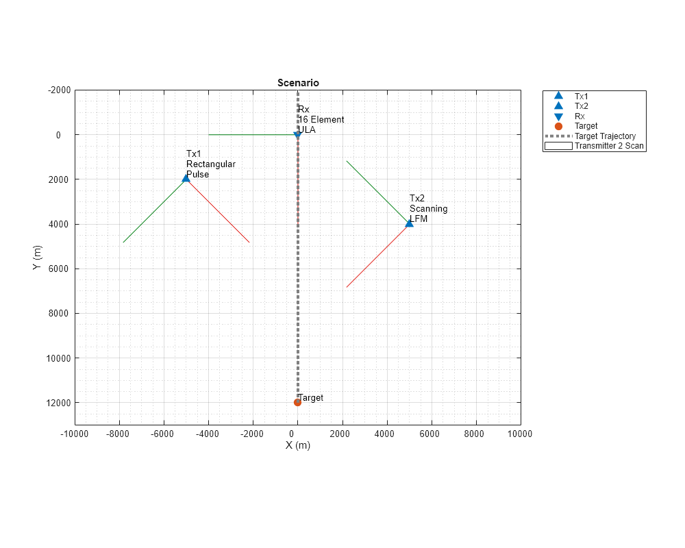

Define Signals of Opportunity

This scenario will define 2 transmitters of opportunity. For this example, the 2 emitters are other active radar systems.

Isotropic Transmitter with Rectangular Waveform

First define a stationary emitter transmitting a rectangular waveform.

% Waveform 1
wav     = phased.RectangularWaveform(PulseWidth=2e-4,PRF=prf1,...
    SampleRate=fs);

Define a transmitter with a peak power of 100 Watts, gain of 20 dB, and loss factor of 6 dB.

% Transmitter 1
tx      = phased.Transmitter(PeakPower=100,Gain=20,LossFactor=6);

Define the transmit antenna as an isotropic antenna element.

% Transmit antenna 1
ant     = phased.IsotropicAntennaElement;
txant   = phased.Radiator(Sensor=ant,PropagationSpeed=c,OperatingFrequency=fc);

Assign the waveform, transmitter, and transmit antenna to the bistaticTransmitter. Set the initial transmission time to 2 times the scenario update time.

% Bistatic transmitter 1: Isotropic transmitter with rectangular waveform
sceneUpdateTime = 1/sceneUpdateRate;
biTx(1) = bistaticTransmitter(InitialTime=2*sceneUpdateTime,Waveform=wav,Transmitter=tx,TransmitAntenna=txant); 

Scanning Array Transmitter with LFM Waveform

Define a scanning emitter transmitting a linear frequency modulated (LFM) waveform.

% Waveform 2
wav = phased.LinearFMWaveform(PulseWidth=1.5e-4,PRF=prf2,...
    SweepBandwidth=bw/2,SampleRate=fs);

Next define a transmitter with a peak power of 500 Watts and a loss factor of 3 dB.

% Transmitter 2
tx      = phased.Transmitter(PeakPower=500,Gain=0,LossFactor=3);

Create a transmit antenna with an 8-element ULA. Set the CombineRadiatedSignals property on the phased.Radiator to false to enable manual scanning of the transmitter. Note the transmitter beamwidth is approximately 12.8 degrees.

% Transmit antenna 2
txarray = phased.ULA(8,lambda/2);
txant   = phased.Radiator(Sensor=txarray,PropagationSpeed=c,OperatingFrequency=fc,CombineRadiatedSignals=false);
biTx2Bw = beamwidth(txarray,fc)

biTx2Bw = 
12.8000

Define a phased.SteeringVector, which will be used to manually scan the transmitter within the simulation loop. The transmitter will electronically scan between -30 and 30 degrees. The scan angle will update every 24 pulses.

% Scanning parameters
pulsesPerScan = 24; % Number of pulses to transmit before updating scan angle
maxScanAng    = 30; % Maximum scan angle (deg) 
scanAngs      = -maxScanAng:5:maxScanAng; % Scan angles (deg) 
numScanAngs   = numel(scanAngs);          % Total number of scans
idxScan       = 8; % Current scan angle index
currentAz     = scanAngs(idxScan)         % Current scan angle (deg), relative to broadside

currentAz = 
5

steervecBiTx2 = phased.SteeringVector(SensorArray=txarray); 

Assign the waveform, transmitter, and transmit antenna to the second bistaticTransmitter. Set the initial transmission time to 5 times the scenario update time.

% Bistatic transmitter 2: Scanning array transmitter with LFM waveform
biTx(2) = bistaticTransmitter(InitialTime=5*sceneUpdateTime,Waveform=wav,Transmitter=tx,TransmitAntenna=txant); 

Configure Bistatic Receiver

Define the receive antenna as a uniform linear array (ULA) with 16 elements spaced a half-wavelength apart. Set the window duration to 0.05 seconds.

% Receive antenna
rxarray = phased.ULA(16,lambda/2);
rxant   = phased.Collector(Sensor=rxarray,...
    PropagationSpeed=c,...
    OperatingFrequency=fc);

% Receiver
rx      = phased.Receiver(Gain=10,SampleRate=fs,NoiseFigure=6,SeedSource='Property');

% Bistatic receiver
winDur  = 0.05;% Window duration (sec)
biRx    = bistaticReceiver(SampleRate=fs,WindowDuration=winDur, ...
    ReceiveAntenna=rxant,Receiver=rx); 

Simulate I/Q Data

Advance the scenario and get the initial time.

advance(scene);
t = scene.SimulationTime;

Transmit and collect pulses for both transmitters for 1 receive window.

% Simulation setup
idxPlats  = 1:4; % All platforms
idxRx     = 3;   % Receiver index
scanCount = 0;   % Scan counter 

% Setup figure for plotting
tl = tiledlayout(figure,2,1);
hAxes = [nexttile(tl) nexttile(tl)]; hold(hAxes,"on");
hTx = gobjects(1,2); 

% Transmit and collect pulses for 1 receive window
hP = helperPlotScenario(txPlat1,txPlat2,rxPlat,tgtPlat); 
for iRxWin = 0:1

Use the nextTime method of the bistaticReceiver to determine the end time of the first bistatic receive window.

    tEnd = nextTime(biRx);

Use the receiver's collect method to initialize the I/Q signal length for the receive window.

    [propSigs,propInfo] = collect(biRx,scene.SimulationTime);

Collect pulses within the receive window.

    while t <= tEnd
        % Get platform positions
        poses = platformPoses(scene);

The platform poses output from the platformPoses method do not include target RCS. Add the rcsSignature objects to the struct.

        % Update poses to include signatures
        poses(1).Signatures = rcsTx1; % Transmitter 1
        poses(2).Signatures = rcsTx2; % Transmitter 2
        poses(4).Signatures = rcsTgt; % Target 

The bistaticFreeSpacePath function creates the bistatic propagation paths. A part of this structure includes the ReflectivityCoefficient, which is the cumulative reflection coefficient for all reflections along the path specified as a scalar magnitude (in linear units). The bistaticFreeSpacePath function derives this value using Kell's Monostatic Bistatic Equivalence Theorem (MBET) approximation and the monostatic rcsSignature.

Consider the following bistatic geometry.

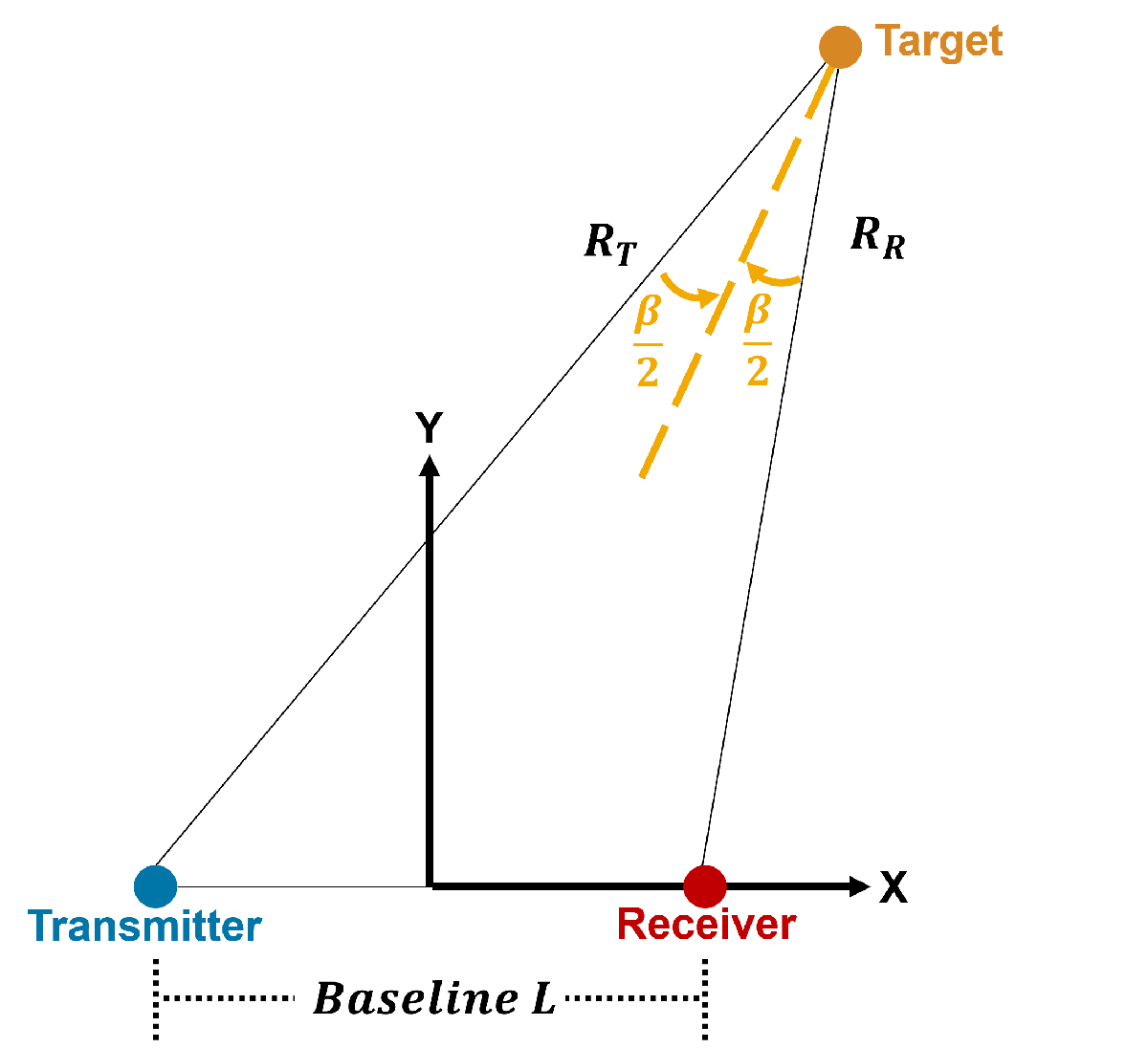
There are 3 paths evident.

• Transmitter-to-receiver: This is also referred to as the direct path or baseline $\mathit{L}$.

• Transmitter-to-target: This is the first leg of the bistatic path and is denoted as ${\mathit{R}}_{\mathit{T}}$ in the diagram above.

• Target-to-receiver: This is the second leg of the bistatic path and is denoted as ${\mathit{R}}_{\mathit{R}}$ in the diagram above.

The bistatic bisector angle is $\beta$. The bistatic range is relative to the direct path and is given by

${\mathit{R}}_{\mathrm{Bistatic}}={\mathit{R}}_{\mathit{T}}+{\mathit{R}}_{\mathit{R}}-\mathit{L}$.

Kell's MBET states that for small bistatic angles (typically less than 5 degrees for more complex targets), the bistatic RCS is equal to the monostatic RCS measured at the bistatic bisector angle $\beta$ and at a frequency $\mathit{f}$ lowered by a factor $\cos \left(\beta /2\right)$.

${\mathrm{RCS}}_{\mathrm{Bistatic}}\left(\beta ,\mathit{f}\right)={\mathrm{RCS}}_{\mathrm{Monostatic}}\left(\beta ,\mathit{f}\cos \left(\beta /2\right)\right)$.

Note that this approximation typically results in overly optimistic bistatic RCS. The true bistatic RCS is typically much lower than the approximation, especially for complex targets. Some cases when this approximation starts to break down are due to changes in:

• Relative Phase between Discrete Scattering Centers: This is analogous to fluctuations in monostatic RCS as target aspect changes. This is typically due to slight changes in bistatic angle.

• Radiation from Discrete Scattering Centers: This occurs when the discrete scattering center reradiates (i.e., retroreflects) energy towards the transmitter and the receiver is on the edge/outside the retroreflected beamwidth.

• Existence of Discrete Scattering Centers: This is typically caused by shadowing.

The MBET approximation is not valid for large bistatic angles, including forward scatter geometry.

If a bistatic RCS pattern is available, the ReflectionCoefficient values can be modified prior to usage by subsequent objects as is done in the Cooperative Bistatic Radar I/Q Simulation and Processing example.

        for iTx = 1:2 % Loop over transmitters
            % Get indices of targets for this transmitter
            idxTgts = (idxPlats ~= iTx) & (idxPlats ~= idxRx); 

            % Calculate paths
            proppaths = bistaticFreeSpacePath(fc, ...
                poses(iTx),poses(idxRx),poses(idxTgts));

            % Transmit
            [txSig,txInfo] = transmit(biTx(iTx),proppaths,t);

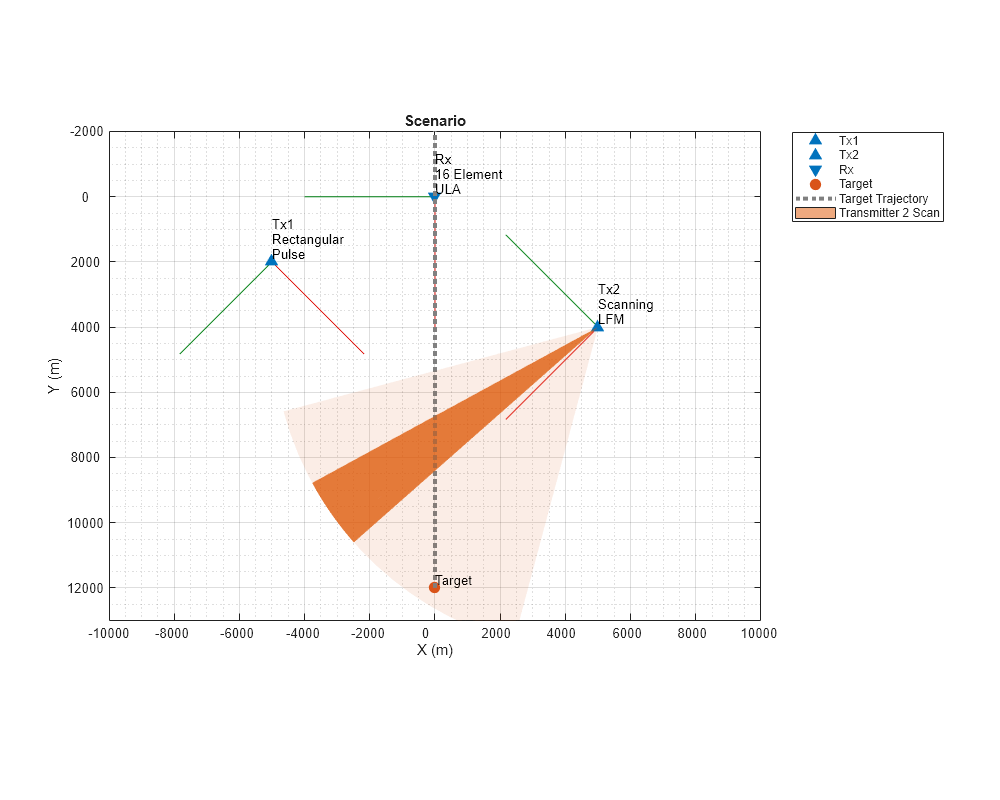
Scan transmitter 2 to the current azimuth angle using the helperGetCurrentAz. Update the scenario plot with helperUpdateScenarioPlot.

            % Scan the transmitter (when applicable)
            if iTx == 2 % If this is transmitter 2

                % Get current scan azimuth angle
                [idxScan,scanCount] = helperGetCurrentAz(biTx(iTx), ...
                    scanAngs,idxScan,scanCount,pulsesPerScan);

                % Steer the transmitter to the current scan azimuth
                sv = steervecBiTx2(fc,[scanAngs(idxScan); 0]);
                txSigCell = txSig;
                txSig = zeros(size(txSig{1},1),numel(proppaths));
                for ip = 1:numel(proppaths)
                    txSig(:,ip) = sv'*txSigCell{ip}.';
                end

                % Update scenario plot to include scan coverage
                sensor = struct('Index',2,'ScanLimits',[-maxScanAng maxScanAng],'FieldOfView',[biTx2Bw;90],...
                    'LookAngle',scanAngs(idxScan),'Range',10e3,'Position',txPlat2.Position,'Orientation',txPlat2.Orientation.');
                helperUpdateScenarioPlot(hP,txPlat1,txPlat2,rxPlat,tgtPlat,sensor);
            end

Collect and accumulate the transmitted pulses. At the accumulate stage, the waveform has been transmitted, propagated, and collected at the receive antenna.

            % Collect transmitted pulses
            collectSigs = collect(biRx,txSig,txInfo,proppaths);

            % Accumulate collected transmissions
            sz = max([size(propSigs);size(collectSigs)],[],1);
            propSigs = paddata(propSigs,sz) + paddata(collectSigs,sz);

Plot the transmitted signal.

            % Plot transmitted signal
            txTimes = (0:(size(txSig,1) - 1))*1/txInfo.SampleRate ...
                + txInfo.StartTime;
            hTx(iTx) = plot(hAxes(1),txTimes,mag2db(max(abs(txSig),[],2)),SeriesIndex=iTx,LineWidth=6);
        end

Advance the scenario to the next update time.

        % Advance the scene
        advance(scene);
        t = scene.SimulationTime;
    end
end

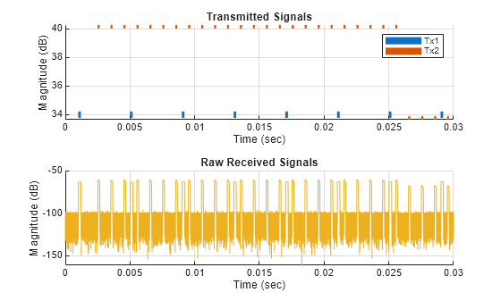
Now that the receive window has been collected, pass the propagated signal through the receiver and plot. The Transmitted Signals plot shows the raw transmissions from the bistaticTransmitter. The higher PRF transmissions are from the scanning radar and are shown in red. The lower PRF transmissions are from the isotropic transmitter and are shown in blue.

The Raw Received Signals plot shows the unprocessed, received I/Q. The pulses that are visible are the direct path returns from each transmitter. Notice that there are 2 distinct direct path returns. The scanning of the second transmitter causes changes in the received magnitude as the signal passes through different lobes of the transmitter's antenna pattern.

In a bistatic radar geometry, the direct path is shorter than a target path, because the direct path travels directly from the transmitter to the receiver, while the target path travels from the transmitter to the target and then from the target to the receiver. This results in a longer overall distance traveled for a target return due to the added "leg". Note that the target is not visible in the raw I/Q without additional processing.

% Receive propagated transmission
[y,rxInfo] = receive(biRx,propSigs,propInfo);

% Plot received signal
rxTimes = (0:(size(y,1) - 1))*1/rxInfo.SampleRate ...
    + rxInfo.StartTime;
plot(hAxes(2),rxTimes,mag2db(abs(sum(y,2))),SeriesIndex=3);

% Label plots
grid(hAxes,"on")
title(hAxes(1),"Transmitted Signals")
legend(hTx,{'Tx1','Tx2'})
title(hAxes(2),"Raw Received Signals")
xlabel(hAxes,"Time (sec)")
ylabel(hAxes,"Magnitude (dB)")
xlim(hAxes(1),[0 0.03])
xlim(hAxes(2),[0 0.03])

Deinterleave Pulses

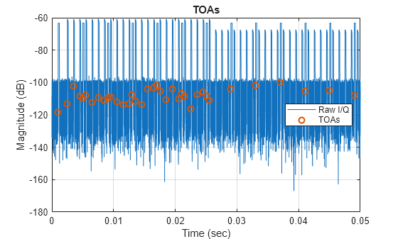
Use the risetime function to get the rising edges, also referred to as leading edges. These edges will be used as times of arrival (TOAs) during deinterleaving.

% Estimate TOAs
[~,toas] = risetime(sum(y,2).*conj(sum(y,2)),fs); 
toas = toas(:).'; % Make sure it is a row vector
idxRise = round(toas*fs); 

% Plot estimated TOAs
figure
plot(rxTimes,mag2db(abs(sum(y,2))))
hold on
grid on
plot(rxTimes(idxRise),mag2db(abs(sum(y(idxRise,:),2))),'o',LineWidth=1.5)
xlabel('Time (sec)')
ylabel('Magnitude (dB)')
legend('Raw I/Q','TOAs',Location='east')
title('TOAs')

Deinterleaving is a process used to separate and identify individual radar pulse trains from a mixture of overlapping pulse trains received at a radar receiver. Deinterleaving can assist with:

• Signal Identification: By analyzing the characteristics of incoming pulses such as Pulse Repetition Interval (PRI), the process identifies which pulses belong to which radar emitter.

• Emitter Classification: Once pulses are grouped, they can be used to classify and identify the type of radar system they originate from, which is essential for situational awareness.

• Efficient Signal Processing: Deinterleaving allows for more efficient processing by reducing the complexity of the signal environment, making it easier to track and analyze specific radar signatures.

Techniques used for pulse deinterleaving include statistical methods, pattern recognition, machine learning, and deep neural networks. Characteristics that can be used for deinterleaving include:

• PRI

• Frequency

• TOA

• Directions of Arrival (DOA)

• Pulse width

This example performs signal identification of the pulse trains using the Sequence Search algorithm. The Sequence Search algorithm is a brute force deinterleaving algorithm that searches for repeating patterns. The algorithm involves calculating the time differences between pulses and identifying intervals that suggest a periodic sequence. Pulses that match an estimated PRI are grouped together and then removed from further consideration. Consider the following example with 2 interleaved sequences.

The algorithm first estimates the PRI using the first two pulses. From there, the estimated PRI is projected forward in time. With each subsequent miss, the tolerance on the PRI is increased.

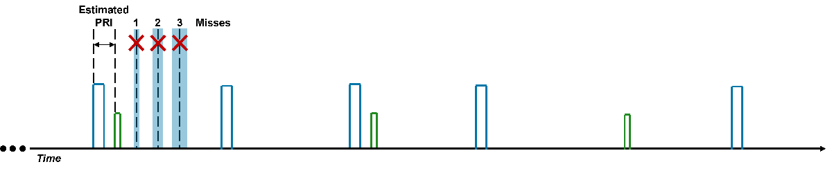
After 3 unsuccessful searches, the algorithm starts again with the next pulse. The estimated PRI is once again projected forward in a similar manner with the tolerance increasing when pulses are missed.

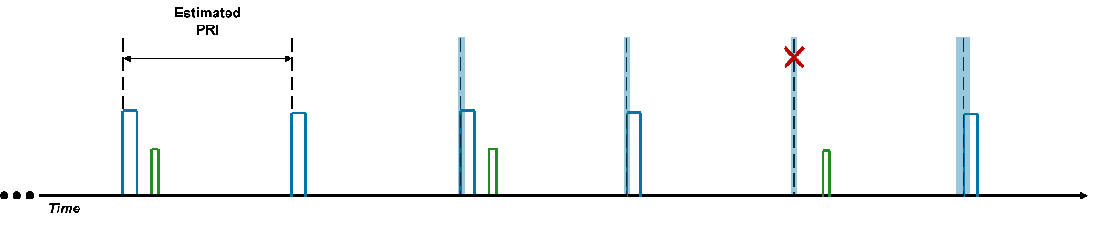
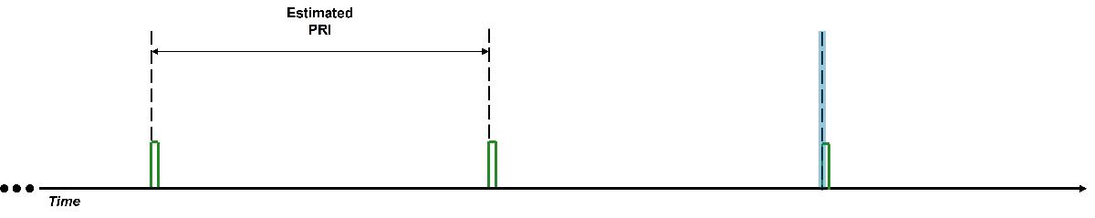
If a sequence is found, the sequence is removed, and the algorithm begins again.

The algorithm proceeds until all sequences are found or all combinations are tried.

The Sequence Search algorithm is most effective in environments where the radar signals have distinct and consistent PRIs. The algorithm suffers when there is too much jitter in the TOA estimation or if there are too many missed pulses. The Sequence Search algorithm can also be used in conjunction with a PRI estimation algorithm like the Sequential Difference (SDIF) or PRI Transform.

Perform deinterleaving using the helperSequenceSeach and plot the identified sequences using helperPlotDeinterleavedSequences.

% Deinterleave
tol = 1/fs*3; 
[id,pris] = helperSequenceSearch(toas,tol);
helperPlotDeinterleavedSequences(rxTimes,y,idxRise,id)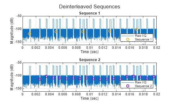

Recall that the initial times for the bistatic transmitters were 0.001 seconds and 0.0025 seconds, respectively. This results in a time difference between the two sequences of 0.0015 seconds.

% Actual difference in start time between the 2 sequences 
initialTimeDiffAct = abs(biTx(1).InitialTime - biTx(2).InitialTime); % Actual time difference (sec)
disp(['Actual time difference (sec) = ' num2str(initialTimeDiffAct)])

Actual time difference (sec) = 0.0015

Note that this difference in start times is evident in the 2 detected sequences. Note that there is a small amount of estimation error.

% Estimate difference in start time between the 2 sequences
id1 = find(id==1,1,'first');
id2 = find(id==2,1,'first');
initialTimeDiffEst = abs(toas(id1) - toas(id2)); % Estimated time difference (sec)
disp(['Estimated time difference (sec) = ' num2str(initialTimeDiffEst)])

Estimated time difference (sec) = 0.0015034

Find the Transmitted Waveforms

In this section, identify the I/Q to use for subsequent bistatic processing and extract the transmitted waveform from the I/Q using helperIsolateSequence. The extracted waveform can be used as a reference for matched filtering. There are many criteria that can be used to identify what is the best waveform for bistatic processing including:

• Ambiguity Function: The waveform should have a favorable ambiguity function, which describes the trade-off between range and Doppler resolution. Ideally, it should have low sidelobes to minimize ambiguity in target detection and localization.

• Bandwidth: A wide bandwidth is generally desirable as it improves range resolution. However, it must be balanced with the available processing capabilities.

• Doppler Tolerance: The waveform should be tolerant to Doppler shifts, which are more pronounced in bistatic configurations due to the relative motion between the transmitter, target, and receiver.

• Synchronization and Timing: In a bistatic setup, maintaining synchronization between the transmitter and receiver is crucial. The waveform should facilitate precise timing and synchronization to ensure accurate target location.

For this example, simply choose the waveform with the highest power, which comes from transmitter 2.

For each sequence identified, the helper blindly performs the following steps:

• Leading Edge Detection: The TOA is assumed to be the leading edge of the reference waveform

• Trailing Edge Detection: A trailing edge is estimated using the falltime function

• Waveform Pulsewidth Estimation: The leading edge and trailing edge indices form the extent of the waveform

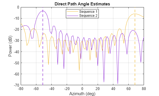
• Direct Path Angle Estimation: The estimated waveform is used to identify the direction of the direct path

• Waveform Refinement: The estimated waveform is further refined by beamforming in the estimated direction of the direct path

• Waveform Selection: Select the sequence with the highest power waveform for further processing

No additional steps are taken by the helper to classify the transmitted waveform and form an ideal matched filter. The noise-contaminated waveform as extracted from the I/Q is used directly in subsequent processing. Note that target contamination of the reference waveform should be minimal, since the received signal of opportunity is both spatially and temporally separated from the target return.

[idxStart,idxStop,refWav,pri,dpAngs] = helperIsolateSequence(biRx,y,id,pris,idxRise);

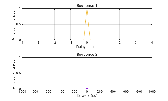
Note that transmitter 2, which is sequence 2 in the plots above, displays a more favorable ambiguity function at a Doppler cut of 0 Hz. For more information about ambiguity functions, see the Waveform Analysis Using the Ambiguity Function example.

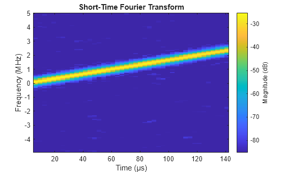
Consider the Short-Time, Fourier Transform of the reference waveform. Note the linear frequency modulation over a sweep bandwidth of approximately 2.5 MHz. The waveform is approximately 140 μs long.

figure
stft(refWav,fs)

Create Bistatic Datacube

Build the bistatic datacube. Typically, a bistatic datacube is zero-referenced to the direct path. This means that the target bistatic range and Doppler will also be relative to the direct path. The bistatic system in this case is stationary, so no zeroing of Doppler is required. Decrease the number of pulses by 1 to prevent an incomplete datacube in the last PRI.

This example does not assume that the transmitter and receiver are time synchronized and only the position of the receiver is known. All subsequent processing will be performed on the bistatic datacube formed in this section.

% Create bistatic datacube
numSamples = round(pri*fs); 
numPulses = floor(numel(idxStart:idxStop)./numSamples);
idxStop = idxStart + numSamples*numPulses - 1; 
numElements = rxarray.NumElements;
yBi = permute(y(idxStart:idxStop,:),[2 1]);
yBi = reshape(yBi,numElements,numSamples,numPulses); 
yBi = permute(yBi,[2 1 3]);

Visualize the bistatic datacube by summing over the antenna elements in the receive array, forming a sum beam at the array broadside. The x-axis is slow time (pulses), and the y-axis is fast-time (samples). The strong direct path return is noticeable close to 0. The other strong, periodic returns are from the other transmitter, which was not selected.

% Visualize bistatic datacube
helperPlotBistaticDatacube(yBi)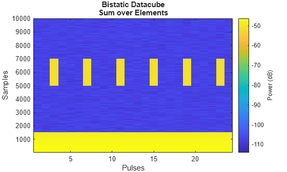

Process Bistatic Datacube

Match Filter and Doppler Process

Perform matched filtering and Doppler processing using the phased.RangeDopplerResponse object. Oversample in Doppler by a factor of 2 and apply a Chebyshev window with 60 dB sidelobes to improve the Doppler spectrum.

% Perform matched filtering and Doppler processing
rngdopresp = phased.RangeDopplerResponse(Mode='Bistatic', ...
    SampleRate=fs, ...
    DopplerWindow='Chebyshev', ...
    DopplerSidelobeAttenuation=60, ...
    DopplerFFTLengthSource='Property', ...
    DopplerFFTLength = size(yBi,3)*2);
mfcoeff = flipud(conj(refWav(:)));
[yBi,rngVec,dopVec] = rngdopresp(yBi,mfcoeff);

The dimensions of the range and Doppler processed datacube is bistatic range-by-number of elements-by-bistatic Doppler. Determine the true bistatic range and Doppler of the target of interest.

% Target range sample
proppaths = bistaticFreeSpacePath(fc, ...
                poses(2),poses(3),poses(4));
tgtRng = proppaths(2).PathLength - proppaths(1).PathLength;
tTgt = range2time(tgtRng/2,c);
timeVec = (0:(numSamples - 1))*1/fs; 
[~,tgtSampleIdx] = min(abs(timeVec - tTgt));

% Target bistatic Doppler
tgtDop = proppaths(2).DopplerShift; 

Plot the range-Doppler response and sum over all elements. Show the true bistatic range and Doppler in the image. Note that the direct path is still very strong and is localized about 0 Doppler due to the fact that the transmitter and receiver are stationary. The direct path has large range sidelobes. The target return is still very difficult to distinguish due to the influence of the direct path. The true target location is shown by the red x.

% Visualize matched filtered and Doppler processed data 
helperPlotRDM(dopVec,rngVec,yBi.*conj(yBi),tgtDop,tgtRng)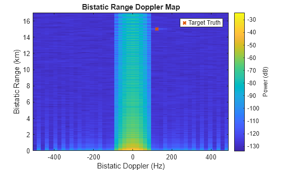

Mitigate Direct Path Interference

The direct path is considered to be a form of interference. Typically, the direct path return is removed. Mitigation strategies for direct path removal include:

• Adding nulls in the direction of the transmitter

• Using a reference beam or antenna

• Adaptive filtering in the spatial/time domain

This example removes the effects of both transmitters by placing nulls in the estimated direction of the transmitters.

First, the beamwidth of the receive array is a little over 6 degrees.

% Receiver beamwidth 
rxBeamwidth = beamwidth(rxarray,fc)

rxBeamwidth = 
6.3600

Specify a series of surveillance beams between -30 and 30 degrees. Space the beams 5 degrees apart in order to minimize scalloping losses.

% Surveillance beams
azSpace = 5; 
azVec = -30:azSpace:30;

Null the beams in the estimated directions of the 2 transmitters.

% Null angle
nullAngs = dpAngs;

% Calculate true target angle index
tgtAz = proppaths(2).AngleOfArrival(1);
[~,tgtBmIdx] = min(abs(azVec - tgtAz(1))); 

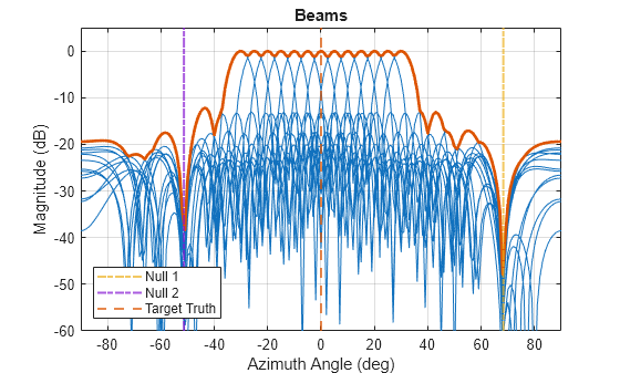
Calculate and plot the surveillance beams using the helper function helperSurveillanceBeams. The effective receiver azimuth pattern is shown as the thick, solid red line. Note that scalloping losses are minimal. The red dashed line indicates the angle of the target. The purple and yellow dot dash lines indicate the null angles in the estimated directions of the direct paths. The transmitters and receiver in this example are stationary. Thus, the beamforming weights only need to be calculated once.

yBF = helperSurveillanceBeams(yBi,azVec,nullAngs,tgtAz);

Plot the datacube in range-angle space and take the max over all Doppler bins. The datacube has now undergone:

• Matched filtering

• Doppler processing

• Beamforming

• Nulling of the direct path

The target is now visible. The true target position is indicated by the red x.

% Plot range-angle after beamforming
helperPlotRAM(azVec,rngVec,yBF,tgtAz(1),tgtRng)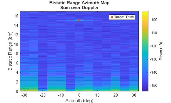 

Now plot the datacube in range-Doppler space and take the sum over all beams. The target is visible and is located where it is expected.

% Plot range-Doppler after beamforming
helperPlotRDM(dopVec,rngVec,yBF,tgtDop,tgtRng)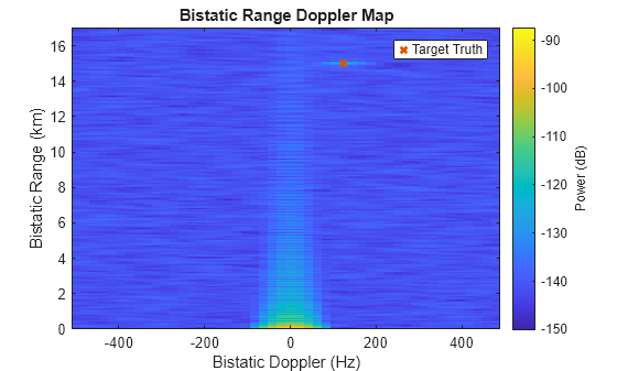

Detect the Target

This section performs the following processing, in the following order, using the helperDetectTargets function:

1. 2 dimensional cell-averaging constant false alarm rate (CA CFAR) detection

2. Clustering using DBSCAN (Density-Based Spatial Clustering of Applications with Noise)

3. Identification of the maximum SNR return in each cluster

4. Parameter estimation

The processing in this section proceeds similarly to the Cooperative Bistatic Radar I/Q Simulation and Processing example. See that example for additional details.

[rngest,dopest,azest] = helperDetectTargets(yBF,rngVec,dopVec,azVec); 

Output the true and estimated bistatic target range, Doppler, and azimuth.

% True target location
Ttrue = table(tgtRng*1e-3,tgtDop,tgtAz(1,:),VariableNames={'Bistatic Range (km)','Bistatic Doppler (m/s)','Azimuth (deg)'});
Ttrue = table(Ttrue,'VariableNames',{'Target Truth'}); 
disp(Ttrue)

                             Target Truth                         
    ______________________________________________________________

    Bistatic Range (km)    Bistatic Doppler (m/s)    Azimuth (deg)
    ___________________    ______________________    _____________
                                                                  
          15.029                   123.28             1.2722e-14  

% Estimated
Test = table(rngest*1e-3,dopest,azest,VariableNames={'Bistatic Range (km)','Bistatic Doppler (m/s)','Azimuth (deg)'});
Test = table(Test,'VariableNames',{'Target Measured'});
disp(Test)

                           Target Measured                        
    ______________________________________________________________

    Bistatic Range (km)    Bistatic Doppler (m/s)    Azimuth (deg)
    ___________________    ______________________    _____________
                                                                  
          15.027                   124.48              0.024964   

Plot the detections in range-Doppler space, taking the sum over all beams. The estimated range, Doppler, and azimuth angle have good agreement with the target truth.

% Plot detections
helperPlotRDM(dopVec,rngVec,yBF,tgtDop,tgtRng,dopest,rngest)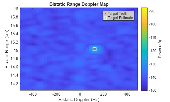

Summary

This example outlines a workflow for the simulation of I/Q for a non-cooperative bistatic system that has 2 different signals of opportunity. It illustrates how to manually scan a bistatic transmitter, deinterleave sequences to form a bistatic datacube, execute range and Doppler processing, mitigate the direct path interference, and conduct target detection and parameter estimation. The demonstrated I/Q simulation and processing techniques can be iteratively applied within a loop to simulate target returns over extended periods.

References

1. Kell, R.E. “On The Derivation of Bistatic RCS from Monostatic Measurements.” Proceedings of the IEEE 53, no. 8 (January 1, 1965): 983–88.

2. Mardia, H.K. “New Techniques for the Deinterleaving of Repetitive Sequences.” IEE Proceedings F Radar and Signal Processing 136, no. 4 (1989): 149.

3. Richards, Mark A. Fundamentals of Radar Signal Processing. 2nd ed. New York: McGraw-Hill education, 2014.

4. Willis, Nicholas J. Bistatic Radar. SciTech Publishing, 2005.

Helpers

helperPlotScenario

function hP = helperPlotScenario(txPlat1,txPlat2,rxPlat,tgtPlat)
% Helper to visualize scenario geometry using theater plotter
% 
% Plots:
%    - Transmitter and receiver orientation
%    - Position of all platforms
%    - Target trajectory 

% Setup theater plotter
hTp = theaterPlot(XLim=[-10 10]*1e3,YLim=[-2 13]*1e3,ZLim=[-15 15]*1e3);
hTpFig = hTp.Parent.Parent;
hTpFig.Units = 'normalized'; 
hTpFig.Position = [0.1 0.1 0.8 0.8];

% Setup plotters:
%   - Orientation plotters
%   - Platform plotters
%   - Trajectory plotters 
%   - Sensor plotter
opTx1 = orientationPlotter(hTp,LocalAxesLength=4e3,MarkerSize=1);
opTx2 = orientationPlotter(hTp,LocalAxesLength=4e3,MarkerSize=1);
opRx = orientationPlotter(hTp,LocalAxesLength=4e3,MarkerSize=1);
plotterTx1 = platformPlotter(hTp,DisplayName='Tx1',Marker='^',MarkerSize=8,MarkerFaceColor=[0 0.4470 0.7410],MarkerEdgeColor=[0 0.4470 0.7410]);
plotterTx2 = platformPlotter(hTp,DisplayName='Tx2',Marker='^',MarkerSize=8,MarkerFaceColor=[0 0.4470 0.7410],MarkerEdgeColor=[0 0.4470 0.7410]);
plotterRx = platformPlotter(hTp,DisplayName='Rx',Marker='v',MarkerSize=8,MarkerFaceColor=[0 0.4470 0.7410],MarkerEdgeColor=[0 0.4470 0.7410]);
plotterTgt = platformPlotter(hTp,DisplayName='Target',Marker='o',MarkerSize=8,MarkerFaceColor=[0.8500 0.3250 0.0980],MarkerEdgeColor=[0.8500 0.3250 0.0980]);
plotterTraj = trajectoryPlotter(hTp,DisplayName='Target Trajectory',LineWidth=3);
plotterSensor = coveragePlotter(hTp,'DisplayName','Transmitter 2 Scan');               
hP = {opTx1, opTx2, opRx, plotterTx1, plotterTx2, plotterRx, plotterTgt, plotterTraj, plotterSensor}; 

% Plot transmitter and receiver orientations
plotOrientation(opTx1,txPlat1.Orientation(3),txPlat1.Orientation(2),txPlat1.Orientation(1),txPlat1.Position)
plotOrientation(opTx2,txPlat2.Orientation(3),txPlat2.Orientation(2),txPlat2.Orientation(1),txPlat2.Position)
plotOrientation(opRx,rxPlat.Orientation(3),rxPlat.Orientation(2),rxPlat.Orientation(1),rxPlat.Position)

% Plot platforms
plotPlatform(plotterTx1,txPlat1.Position,txPlat1.Trajectory.Velocity,{['Tx1' newline 'Rectangular' newline 'Pulse']});
plotPlatform(plotterTx2,txPlat2.Position,txPlat2.Trajectory.Velocity,{['Tx2' newline 'Scanning' newline 'LFM']});
plotPlatform(plotterRx,rxPlat.Position,rxPlat.Trajectory.Velocity,{['Rx' newline '16 Element' newline 'ULA']});
plotPlatform(plotterTgt,tgtPlat.Position,tgtPlat.Trajectory.Velocity,{'Target'});

% Plot target trajectory 
plotTrajectory(plotterTraj,{(tgtPlat.Position(:) + tgtPlat.Trajectory.Velocity(:).*linspace(0,5000,3)).'})
grid('on')
title('Scenario')
view([0 90])
pause(0.1)
end

helperUpdateScenarioPlot

function helperUpdateScenarioPlot(hP,txPlat1,txPlat2,rxPlat,tgtPlat,sensor)
% Helper to update scenario theaterPlot
%
% hP = {opTx1, opTx2, opRx, plotterTx1, plotterTx2, plotterRx, ...
%    plotterTgt, plotterTraj, plotterSensor}

% Plot transmitter and receiver orientations
plotOrientation(hP{1},txPlat1.Orientation(3),txPlat1.Orientation(2),txPlat1.Orientation(1),txPlat1.Position)
plotOrientation(hP{2},txPlat2.Orientation(3),txPlat2.Orientation(2),txPlat2.Orientation(1),txPlat2.Position)
plotOrientation(hP{3},rxPlat.Orientation(3),rxPlat.Orientation(2),rxPlat.Orientation(1),rxPlat.Position)

% Plot platforms
plotPlatform(hP{4},txPlat1.Position,txPlat1.Trajectory.Velocity,{['Tx1' newline 'Rectangular' newline 'Pulse']});
plotPlatform(hP{5},txPlat2.Position,txPlat2.Trajectory.Velocity,{['Tx2' newline 'Scanning' newline 'LFM']});
plotPlatform(hP{6},rxPlat.Position,rxPlat.Trajectory.Velocity,{['Rx' newline '16 Element' newline 'ULA']});
plotPlatform(hP{7},tgtPlat.Position,tgtPlat.Trajectory.Velocity,{'Target'});

% Plot target trajectory 
plotTrajectory(hP{8},{(tgtPlat.Position(:) + tgtPlat.Trajectory.Velocity(:).*linspace(0,5000,3)).'})

% Sensor 
plotCoverage(hP{9},sensor)
pause(0.1)
end

helperGetCurrentAz

function [idxScan,scanCount] = helperGetCurrentAz(biTx,scanAngs,idxScan,scanCount,scanPulses)
% Helper returns current scan index and scan count

numAngs = length(scanAngs); 
if biTx.IsTransmitting
    scanCount = scanCount + 1;
    % Update scan angle
    if scanCount == (scanPulses + 1)
        scanCount = 1;
        idxScan = mod(idxScan + 1,numAngs);
        idxScan(idxScan == 0) = numAngs;
    end
end
end

helperPlotBistaticDatacube

function helperPlotBistaticDatacube(yBi)
% Helper plots the bistatic datacube

numSamples = size(yBi,1);
numPulses = size(yBi,3); 

% Plot bistatic datacube 
figure()
imagesc(1:numPulses,1:numSamples,pow2db(abs(squeeze(sum(yBi.*conj(yBi),2)))))
axis xy
hold on

% Label
xlabel('Pulses')
ylabel('Samples')
title(sprintf('Bistatic Datacube\nSum over Elements'))

% Colorbar
hC = colorbar;
hC.Label.String = 'Power (dB)';
end

helperPlotDeinterleavedSequences

function helperPlotDeinterleavedSequences(rxTimes,y,idxRise,id)
% Helper to plot identified sequences

% Plot identified sequences
uIDs   = unique(id);  % Unique IDs
numSeq = numel(uIDs); % Number of sequences
tiledlayout(figure,numSeq,1);
for ii = 1:numSeq
    idx = find(id == uIDs(ii));
    nexttile; 
    plot(rxTimes,mag2db(abs(sum(y,2))));
    hold on
    plot(rxTimes(idxRise(idx)),mag2db(abs(sum(y(idxRise(idx),:),2))),'o',LineWidth=1.5,SeriesIndex=ii+2)
    grid on
    xlabel('Time (sec)')
    ylabel('Magnitude (dB)')
    xlim([0 0.02])
    sequenceName = sprintf('Sequence %d',ii);
    legend({'Raw I/Q' sequenceName},Location='southeast')
    title(sequenceName)
end
sgtitle('Deinterleaved Sequences')
end

helperIsolateSequence

function [idxStart,idxStop,refWav,pri,dpAngs] = helperIsolateSequence(biRx,y,id,pris,idxRise)
% Helper returns:
%   - Start/stop indices of selected sequence
%   - Reference waveform for matched filtering
%   - PRI estimate of selected sequence
%   - Direct path angle of selected emitter
%   - Direct path angles for all estimated emitters
%
% Helper plots: 
%   - Direct path angle estimates for all emitters
%   - Ambiguity function at 0 Doppler for all emitters 

uIDs   = unique(id);
numSeq = numel(uIDs);
yPwr   = sum(y,2).*conj(sum(y,2));

% Get parameters from bistatic receiver
fs = biRx.SampleRate; 
fc = biRx.ReceiveAntenna.OperatingFrequency;
rxarray = biRx.ReceiveAntenna.Sensor; 

% Initialize
idxPulseStart = zeros(1,numSeq); % Pulse start index
idxPulseStop  = zeros(1,numSeq); % Pulse stop index
idxStart      = zeros(1,numSeq); % Pulse train sequence start index
idxStop       = zeros(1,numSeq); % Pulse train sequence stop index
maxPwr        = zeros(1,numSeq); % Maximum power (dB)
pri           = zeros(1,numSeq); % Sequence PRI (sec)

% Determine falling edges
for ii = 1:numSeq
    % Get indices for a single PRI 
    idx = find(id == uIDs(ii));
    thisPRI = round(pris(idx(1))*fs)*1/fs;
    pri(ii) = thisPRI;
    idxStart(ii) = idxRise(idx(1));
    idxStop(ii) = min(round(idxRise(idx(end)) + pri(ii)*fs),size(y,1));
    idxSeq = idxStart(ii):idxStop(ii);
    idxPulseStart(ii) = idxRise(idx(1));
    idxPRI = round(idxStart(ii) + pri(ii)*fs); 

    % Identify falling edge 
    [~,lt] = falltime(yPwr(idxStart(ii):idxPRI),fs);  
    idxFall = round(lt*fs);  
    idxPulseStop(ii) = idxSeq(idxFall(1)); 
    maxPwr(ii) = max(yPwr(idxPulseStart(ii):idxPulseStop(ii))); 
end

% Create steering vectors for direct path search
azSpace = 2;
azVec = -80:azSpace:80;
steervecBiRx = phased.SteeringVector(SensorArray=rxarray);
sv = steervecBiRx(fc,[azVec; zeros(size(azVec))]);

% Setup figure
figure
dpAngs = zeros(2,numSeq);
hP = gobjects(1,numSeq); 
for ii = 1:numSeq
    % Lay down beams
    yBF = sv'*y(idxPulseStart(ii):idxPulseStop(ii),:).'; % Use the identified waveforms
    yBFPwr = yBF.*conj(yBF);

    % Assume that maximum is the direction of the direct path for this
    % waveform
    [~,idxAng] = max(sum(yBFPwr,2));
    [~,dpAz] = refinepeaks(sum(yBFPwr,2),idxAng,azVec);
    dpAngs(:,ii) = [dpAz; 0];

    % Plot for selected sequence
    hP(ii) = plot(azVec,pow2db(sum(yBFPwr,2)),SeriesIndex=ii+2);
    hold on
    grid on
    xline(dpAz,'--',LineWidth=1.5,SeriesIndex=ii+2)

end
xlabel('Azimuth (deg)')
ylabel('Power (dB)')
title('Direct Path Angle Estimates')
legend(hP,arrayfun(@(x) sprintf('Sequence %d',x),1:numSeq,UniformOutput=false),Location="best")

% Plot ambiguity function at 0 Doppler 
figure
tiledlayout(numSeq,1);
for ii = 1:numSeq
    refWav = y(idxPulseStart(ii):idxPulseStop(ii),:);
    sv = steervecBiRx(fc,dpAngs(:,ii)); 
    refWav = sv'*refWav.'; 
    nexttile
    ambgfun(paddata(refWav,[1 round(fs*pri(ii))]),fs,1/pri(ii),Cut='Doppler')
    hAxes = gca; 
    hAxes.Children.SeriesIndex = ii + 2; 
    title(sprintf('Sequence %d',ii))
end

% Use the waveform with the most power for subsequent processing
[~,idxUse] = max(maxPwr);

% Get selected waveform
refWav = y(idxPulseStart(idxUse):idxPulseStop(idxUse),:);
sv = steervecBiRx(fc,dpAngs(idxUse)); 
refWav = sv'*refWav.'; 

% Set outputs for selected sequence
idxStart = idxStart(idxUse); 
idxStop = idxStop(idxUse); 
pri = pri(idxUse); 
end

helperPlotRDM

function helperPlotRDM(dopVec,rngVec,resp,tgtDop,tgtRng,dopest,rngest)
% Helper to plot the range-Doppler map
%   - Includes target range and Doppler
%   - Optionally includes estimated range and Doppler
%
% Sums over elements or beams

% Plot RDM
figure
imagesc(dopVec,rngVec*1e-3,pow2db(abs(squeeze(sum(resp,2)))))
axis xy
hold on

% Plot target truth
plot(tgtDop,tgtRng*1e-3,'x',SeriesIndex=2,LineWidth=2)

% Colorbar
hC = colorbar;
hC.Label.String = 'Power (dB)';

% Labels
xlabel('Bistatic Doppler (Hz)')
ylabel('Bistatic Range (km)')

% Plot title 
title('Bistatic Range Doppler Map')

% Optionally plot estimated range and Doppler 
if nargin == 7
    plot(dopest,rngest*1e-3,'sw',LineWidth=2,MarkerSize=10)
    ylim([tgtRng - 1e3 tgtRng + 1e3]*1e-3)
    legend('Target Truth','Target Estimate',Color=[0.8 0.8 0.8])
else
    ylim([0 tgtRng + 2e3]*1e-3)
    legend('Target Truth');
end
pause(0.1)
end

helperSurveillanceBeams

function yBF = helperSurveillanceBeams(yBi,azVec,nullAngs,tgtAz)
% Helper:
%    - Calculates surveillance beams with user-requested nulls
%    - Plots surveillance beams
%    - Outputs beamformed datacube <bistatic range> x <beams> x <bistatic Doppler>
%
% Note that the output is power in units of Watts. 

% Calculate surveillance beams
azSpace = azVec(2) - azVec(1); 
[numSamples,numElements,numDop] = size(yBi);
pos = (0:numElements - 1).*0.5;
numBeams = numel(azVec);
yBF = zeros(numBeams,numSamples*numDop);
yBi = permute(yBi,[2 1 3]); % <elements> x <bistatic range> x <bistatic Doppler>
yBi = reshape(yBi,numElements,[]); % <elements> x <bistatic range>*<bistatic Doppler>
afAng = -90:90;
af = zeros(numel(afAng),numBeams); 
for ib = 1:numBeams
    if any(~((azVec(ib) - azSpace) < nullAngs(1,:) & nullAngs(1,:) < (azVec(ib) + azSpace)))
        
        wts = minvarweights(pos,azVec(ib),NullAngle=nullAngs);

        % Plot the array factor 
        af(:,ib) = arrayfactor(pos,afAng,wts);

        % Beamform
        yBF(ib,:) = wts'*yBi;
    end
end

% Plot beams
helperPlotBeams(afAng,af,nullAngs,tgtAz)

% Reshape datacube
yBF = reshape(yBF,numBeams,numSamples,numDop); % <beams> x <bistatic range> x <bistatic Doppler>
yBF = permute(yBF,[2 1 3]); %  <bistatic range> x <beams> x <bistatic Doppler>

% Convert to power
yBF = yBF.*conj(yBF); 

end

helperPlotBeams

function helperPlotBeams(afAng,af,nullAngs,tgtAng) 
% Helper to plot:
%    - Surveillance beams
%    - Null angles
%    - Target angle

% Plot array factor 
figure;
hArrayAxes = axes; 
plot(hArrayAxes,afAng,mag2db(abs(af)),SeriesIndex=1)
hold on
grid on
axis tight
ylim([-60 5])

% Plot array max 
azMax = max(mag2db(abs(af)),[],2);
h(1) = plot(hArrayAxes,afAng,azMax,LineWidth=2,SeriesIndex=2);

% Label
xlabel('Azimuth Angle (deg)')
ylabel('Magnitude (dB)')
title('Beams')

% Null angle in direction of direct path 
h(1) = xline(nullAngs(1,1),'-.',LineWidth=1.5,SeriesIndex=3);
if size(nullAngs,2) > 1
    h(2) = xline(nullAngs(1,2),'-.',LineWidth=1.5,SeriesIndex=4);
end

% Target angle
h(3) = xline(tgtAng(1),'--',LineWidth=1.5,SeriesIndex=2);
legend(h,{'Null 1','Null 2','Target Truth'},Location='southwest')
pause(0.1)
end

helperPlotRAM

function helperPlotRAM(azVec,rngVec,yPwr,tgtAng,tgtRng)
% Helper to plot the range-angle map
%   - Includes target range and Doppler
%
% Max over Doppler

% Plot RAM
figure
imagesc(azVec,rngVec*1e-3,pow2db(abs(squeeze(max(yPwr,[],3)))))
axis xy
hold on

% Plot target truth
plot(tgtAng,tgtRng*1e-3,'x',SeriesIndex = 2,LineWidth=2)
ylim([0 tgtRng + 2e3]*1e-3)

% Labels
xlabel('Azimuth (deg)')
ylabel('Bistatic Range (km)')
title(sprintf('Bistatic Range Azimuth Map\nSum over Doppler'))
legend('Target Truth')

% Colorbar
hC = colorbar;
hC.Label.String = 'Power (dB)';
pause(0.1)
end

helperDetectTargets

function [rngest,dopest,azest] = helperDetectTargets(yBF,rngVec,dopVec,azVec)
% This helper does the following: 
%    1. 2D CA CFAR
%    2. DBSCAN Clustering
%    3. Max SNR of Cluster
%    4. Parameter Estimation 

% 1. 2D CA CFAR
numGuardCells    = [10 5]; % Number of guard cells for each side
numTrainingCells = [10 5]; % Number of training cells for each side
Pfa              = 1e-8;  % Probability of false alarm
cfar = phased.CFARDetector2D(GuardBandSize=numGuardCells, ...
    TrainingBandSize=numTrainingCells, ...
    ProbabilityFalseAlarm=Pfa, ...
    NoisePowerOutputPort=true, ...
    OutputFormat='Detection index');

% Perform 2D CFAR detection
[dets,noise] = helperCFAR(cfar,yBF); 

% 2. DBSCAN Clustering
clust = clusterDBSCAN(Epsilon=1,MinNumPoints=5);
idxClust = clust(dets.');

% 3. Max SNR of Cluster
detsClust = helperDetectionMaxSNR(yBF,dets,noise,idxClust);

% 4. Parameter Estimation 

% Refine detection estimates in range and Doppler
rangeEstimator = phased.RangeEstimator; 
dopEstimator = phased.DopplerEstimator;
rngest = rangeEstimator(yBF,rngVec(:),detsClust);
dopest = dopEstimator(yBF,dopVec,detsClust);

% Refine azimuth estimate
[~,azest] = refinepeaks(yBF,detsClust.',azVec,Dimension=2);
end

helperCFAR

function [dets,noise] = helperCFAR(cfar,yPwr)
% Helper to determine CUT indices, as well as perform 2D CFAR detection over
% beams

numGuardCells = cfar.GuardBandSize;
numTrainingCells = cfar.TrainingBandSize;

% Determine cell-under-test (CUT) indices
[numSamples,numBeams,numDop] = size(yPwr); 
numCellsRng       = numGuardCells(1) + numTrainingCells(1); 
idxCUTRng         = (numCellsRng+1):(numSamples - numCellsRng);  % Range indices of cells under test (CUT) 
numCellsDop       = numGuardCells(2) + numTrainingCells(2); 
idxCUTDop         = (numCellsDop + 1):(numDop - numCellsDop); % Doppler indices of cells under test (CUT) 
[idxCUT1,idxCUT2] = meshgrid(idxCUTRng,idxCUTDop);
idxCUT = [idxCUT1(:) idxCUT2(:)].';

% Perform CFAR detection over beams 
dets = []; 
noise = []; 
for ib = 1:numBeams % Perform detection over beams 
    [detTmp,noiseTmp] = cfar(squeeze(yPwr(:,ib,:)),idxCUT);
    beamTmp = ib.*ones(1,size(detTmp,2)); 
    detTmp = [detTmp(1,:); beamTmp; detTmp(2,:)];
    dets = [dets detTmp]; %#ok<AGROW>
    noise = [noise noiseTmp]; %#ok<AGROW>
end
end

helperDetectionMaxSNR

function [detsClust,snrest] = helperDetectionMaxSNR(yPwr,dets,noise,idxClust)
% Helper that outputs the maximum SNR detection in each cluster

idxU = unique(idxClust(idxClust~=-1)); % Unique clusters that are not noise
detsClust = [];
snrest = [];
for iu = 1:numel(idxU)
    idx = find(idxClust == idxU(iu));

    % Find max SNR
    linidx = sub2ind(size(yPwr),dets(1,idx),dets(2,idx),dets(3,idx));
    snrs = yPwr(linidx)./noise(:,idx);
    [~,idxMax] = max(snrs);

    % Save dets
    detsClust = [detsClust [dets(1,idx(idxMax));dets(2,idx(idxMax));dets(3,idx(idxMax))]]; %#ok<AGROW>
    snrest = [snrest yPwr(linidx(idxMax))./noise(:,idx(idxMax))]; %#ok<AGROW>
end
snrest = pow2db(snrest); 
end