Main Content

step

Step response of dynamic system

Description

step computes the step response to a step change in input value from U to U + dU after td time units.
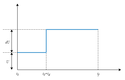
Step response plot characterized by start time, final time, baseline input, step amplitude, and time delay.

Here,

  • t0 is the simulation start time.

  • td is the step delay.

  • U is the baseline input value or bias.

  • dU is the step amplitude.

By default, the function applies step for t0 = 0, U = 0, dU = 1, and td = 0. But, you can configure these values using RespConfig. You can also specify the initial state x(t0). When you don't specify the initial state, step assumes the system is initially at rest with input level U.

[y,tOut] = step(sys) computes the step response y of dynamic system sys. step automatically determines the time steps and duration of the simulation based on the system dynamics.

[y,tOut] = step(sys,t) simulates the response for the time steps specified by t. To define the time steps, you can specify:

  • The final simulation time using a scalar value.

  • The initial and final simulation times using a two-element vector. (since R2023b)

  • All the time steps using a vector.

[y,tOut] = step(sys,t,p) specifies the parameter trajectory p for linear parameter-varying (LPV) models. (since R2023a)

[y,tOut,x] = step(___) also returns the state trajectories x, when sys is a state-space model, such as an ss or idss model.

[y,tOut,x,ysd] = step(___) returns the standard deviation of the step response for identified models. This syntax requires System Identification Toolbox™ software.

[y,tOut,x,~,pOut] = step(sys,t,p) returns the parameter trajectories for LPV models. (since R2023a)

[y,tOut] = step(___,config) specifies additional options for computing the step response, such as the step amplitude or input offset. Use RespConfig to create config.

example

step(___) plots the step response of sys with default plotting options for all of the previous input argument combinations. For more plot customization options, use stepplot.

  • To plot responses for multiple dynamic systems on the same plot, you can specify sys as a comma-separated list of models. For example, step(sys1,sys2,sys3) plots the responses for three models on the same plot.

  • To specify a color, line style, and marker for each system in the plot, specify a LineSpec value for each system. For example, step(sys1,LineSpec1,sys2,LineSpec2) plots two models and specifies their plot style. For more information on specifying a LineSpec value, see stepplot.

Examples

collapse all

Plot the step response of a continuous-time system represented by the following transfer function.

sys(s)=4s2+2s+10.

For this example, create a tf model that represents the transfer function. You can similarly plot the step response of other dynamic system model types, such as zero-pole gain (zpk) or state-space (ss) models.

sys = tf(4,[1 2 10]);

Plot the step response.

step(sys)

MATLAB figure

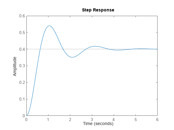
The step plot automatically includes a dotted horizontal line indicating the steady-state response. In a MATLAB® figure window, you can right-click on the plot to view other step-response characteristics such as peak response and settling time. For more information about these characteristics, see stepinfo.

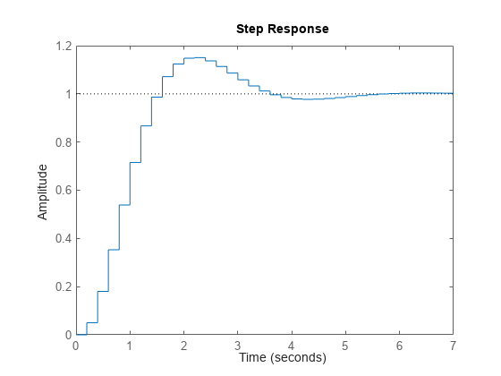
Plot the step response of a discrete-time system. The system has a sample time of 0.2 s and is represented by the following state-space matrices.

A = [1.6 -0.7;
      1  0];
B = [0.5; 0];
C = [0.1 0.1];
D = 0;

Create the state-space model and plot its step response.

sys = ss(A,B,C,D,0.2);
step(sys)

MATLAB figure

The step response reflects the discretization of the model, showing the response computed every 0.2 seconds.

Examine the step response of the following transfer function.

sys = zpk(-1,[-0.2+3j,-0.2-3j],1) * tf([1 1],[1 0.05]) 
sys =
 
            (s+1)^2
  ----------------------------
  (s+0.05) (s^2 + 0.4s + 9.04)
 
Continuous-time zero/pole/gain model.
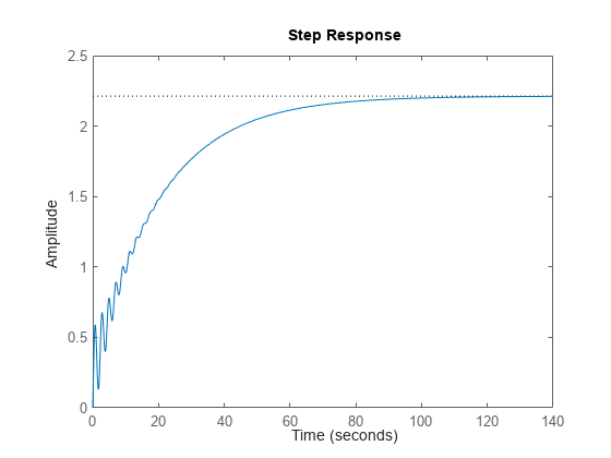
step(sys)

MATLAB figure

By default, step chooses an end time that shows the steady state that the response is trending toward. This system has fast transients, however, which are obscured on this time scale. To get a closer look at the transient response, limit the step plot to t = 15 s.

step(sys,15)

MATLAB figure

Alternatively, you can specify the exact times at which you want to examine the step response, provided they are separated by a constant interval. For instance, examine the response from the end of the transient until the system reaches steady state.

t = 20:0.2:120;
step(sys,t)

MATLAB figure

Even though this plot begins at t = 20, step always applies the step input at t = 0.

Consider the following second-order state-space model:

[x˙1x˙2]=[-0.5572-0.78140.78140][x1x2]+[1-102][u1u2]y=[1.96916.4493][x1x2]

A = [-0.5572,-0.7814;0.7814,0];
B = [1,-1;0,2];
C = [1.9691,6.4493];
sys = ss(A,B,C,0);

This model has two inputs and one output, so it has two channels: from the first input to the output, and from the second input to the output. Each channel has its own step response.

When you use step, it computes the responses of all channels.

step(sys)

MATLAB figure

The left plot shows the step response of the first input channel, and the right plot shows the step response of the second input channel. Whenever you use step to plot the responses of a MIMO model, it generates an array of plots representing all the I/O channels of the model. For instance, create a random state-space model with five states, three inputs, and two outputs, and plot its step response.

sys = rss(5,2,3);
step(sys)

MATLAB figure

In a MATLAB figure window, you can restrict the plot to a subset of channels by right-clicking on the plot and selecting I/O Selector.

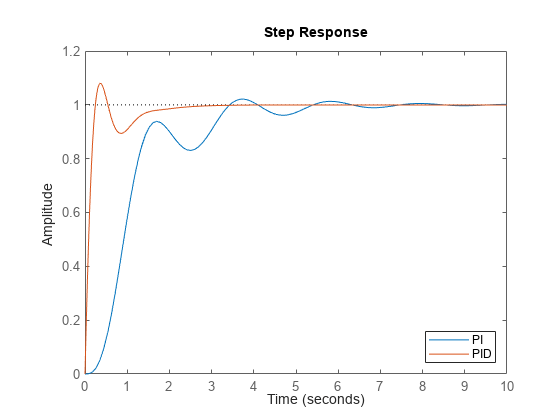
step allows you to plot the responses of multiple dynamic systems on the same axis. For instance, compare the closed-loop response of a system with a PI controller and a PID controller. Create a transfer function of the system and tune the controllers.

H = tf(4,[1 2 10]);
C1 = pidtune(H,'PI');
C2 = pidtune(H,'PID');

Form the closed-loop systems and plot their step responses.

sys1 = feedback(H*C1,1);
sys2 = feedback(H*C2,1);
step(sys1,sys2)
legend('PI','PID','Location','SouthEast')

MATLAB figure

By default, step chooses distinct colors for each system that you plot. You can specify colors and line styles using the LineSpec input argument.

 step(sys1,'r--',sys2,'b')
 legend('PI','PID','Location','SouthEast')

MATLAB figure

The first LineSpec 'r--' specifies a dashed red line for the response with the PI controller. The second LineSpec 'b' specifies a solid blue line for the response with the PID controller. The legend reflects the specified colors and linestyles. For more plot customization options, use stepplot.

The example Compare Responses of Multiple Systems shows how to plot responses of several individual systems on a single axis. When you have multiple dynamic systems arranged in a model array, step plots all their responses at once.

Create a model array. For this example, use a one-dimensional array of second-order transfer functions having different natural frequencies. First, preallocate memory for the model array. The following command creates a 1-by-5 row of zero-gain SISO transfer functions. The first two dimensions represent the model outputs and inputs. The remaining dimensions are the array dimensions.

 sys = tf(zeros(1,1,1,5));

Populate the array.

w0 = 1.5:1:5.5;    % natural frequencies
zeta = 0.5;        % damping constant
for i = 1:length(w0)
   sys(:,:,1,i) = tf(w0(i)^2,[1 2*zeta*w0(i) w0(i)^2]);
end

(For more information about model arrays and how to create them, see Model Arrays.) Plot the step responses of all models in the array.

step(sys)

MATLAB figure

step uses the same linestyle for the responses of all entries in the array. One way to distinguish among entries is to use the SamplingGrid property of dynamic system models to associate each entry in the array with the corresponding w0 value.

sys.SamplingGrid = struct('frequency',w0);

Now, when you plot the responses in a MATLAB figure window, you can click a trace to see which frequency value it corresponds to.

When you give it an output argument, step returns an array of response data. For a SISO system, the response data is returned as a column vector of length equal to the number of time points at which the response is sampled. You can provide the vector t of time points, or allow step to select time points for you based on system dynamics. For instance, extract the step response of a SISO system at 101 time points between t = 0 and t = 5 s.

sys = tf(4,[1 2 10]);
t = 0:0.05:5;
y = step(sys,t);
size(y)
ans = 1×2

   101     1

For a MIMO system, the response data is returned in an array of dimensions N-by-Ny-by-Nu, where Ny and Nu are the number of outputs and inputs of the dynamic system. For instance, consider the following state-space model, representing a two-input, one-output system.

A = [-0.5572,-0.7814;0.7814,0];
B = [1,-1;0,2];
C = [1.9691,6.4493];
sys = ss(A,B,C,0);

Extract the step response of this system at 200 time points between t = 0 and t = 20 s.

t = linspace(0,20,200);
y = step(sys,t);
size(y)
ans = 1×3

   200     1     2

y(:,i,j) is a column vector containing the step response from the jth input to the ith output at the times t. For instance, extract the step response from the second input to the output.

y12 = y(:,1,2);
plot(t,y12)

Figure contains an axes object. The axes object contains an object of type line.

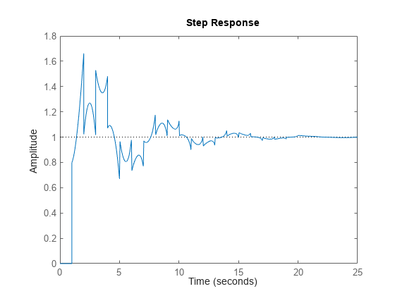
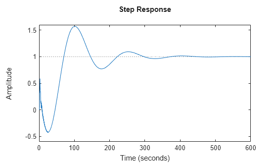
Create a feedback loop with delay and plot its step response.

s = tf('s');
G = exp(-s) * (0.8*s^2+s+2)/(s^2+s);
sys = feedback(ss(G),1);
step(sys)

MATLAB figure

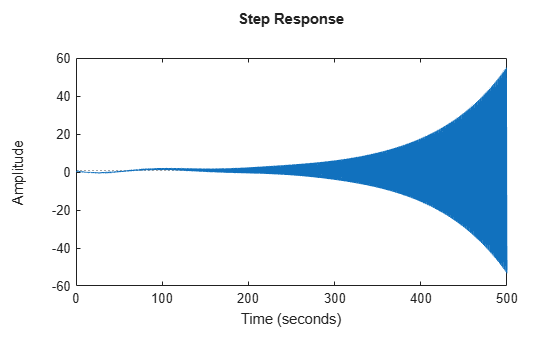
The system step response displayed is chaotic. The step response of systems with internal delays may exhibit odd behavior, such as recurring jumps. Such behavior is a feature of the system and not software anomalies.

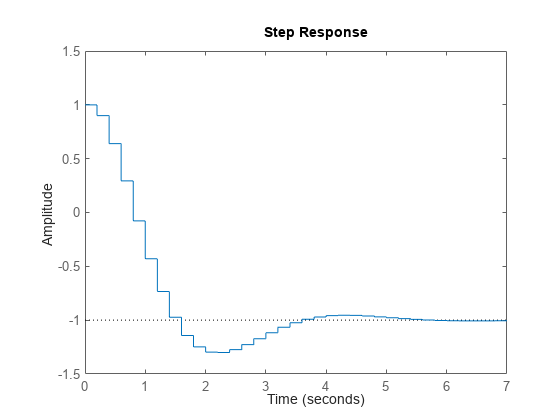
By default, step applies an input signal that changes from 0 to 1 at t = 0. To customize the amplitude and bias, use RespConfig. For instance, compute the response of a SISO state-space model to a signal that changes from 1 to –1 to at t = 0.

A = [1.6 -0.7;
      1  0];
B = [0.5; 0];
C = [0.1 0.1];
D = 0;
sys = ss(A,B,C,D,0.2);

opt = RespConfig;
opt.Bias = 1;
opt.Amplitude = -2;

step(sys,opt)

MATLAB figure

For responses to arbitrary input signals, use lsim.

Compare the step response of a parametric identified model to a non-parametric (empirical) model. Also view their 3 σ confidence regions.

Load the data.

load iddata1 z1

Estimate a parametric model.

sys1 = ssest(z1,4);

Estimate a non-parametric model.

sys2 = impulseest(z1);

Plot the step responses for comparison.

t = (0:0.1:10)';
[y1, ~, ~, ysd1] = step(sys1,t);
[y2, ~, ~, ysd2] = step(sys2,t);
plot(t, y1, 'b', t, y1+3*ysd1, 'b:', t, y1-3*ysd1, 'b:')
hold on
plot(t, y2, 'g', t, y2+3*ysd2, 'g:', t, y2-3*ysd2, 'g:')

Figure contains an axes object. The axes object contains 6 objects of type line.

Compute the step response of an identified time-series model.

A time-series model, also called a signal model, is one without measured input signals. The step plot of this model uses its (unmeasured) noise channel as the input channel to which the step signal is applied.

Load the data.

load iddata9;

Estimate a time-series model.

sys = ar(z9, 4);

sys is a model of the form A y(t) = e(t) , where e(t) represents the noise channel. For computation of step response, e(t) is treated as an input channel, and is named e@y1.

Plot the step response.

step(sys)

MATLAB figure

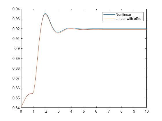
Validate the linearization of a nonlinear ARX model by comparing the small amplitude step responses of the linear and nonlinear models.

Load the data.

load iddata2 z2;

Estimate a nonlinear ARX model.

nlsys = nlarx(z2,[4 3 10],idTreePartition,'custom',...
    {'sin(y1(t-2)*u1(t))+y1(t-2)*u1(t)+u1(t).*u1(t-13)',...
    'y1(t-5)*y1(t-5)*y1(t-1)'},'nlr',[1:5, 7 9]);

Determine an equilibrium operating point for nlsys corresponding to a steady-state input value of 1.

u0 = 1;
[X,~,r] = findop(nlsys, 'steady', 1);
y0 = r.SignalLevels.Output;

Obtain a linear approximation of nlsys at this operating point.

sys = linearize(nlsys,u0,X);

Validate the usefulness of sys by comparing its small-amplitude step response to that of nlsys.

The nonlinear system nlsys is operating at an equilibrium level dictated by (u0,y0). Introduce a step perturbation of size 0.1 about this steady-state and compute the corresponding response.

opt = RespConfig;
opt.InputOffset = u0;
opt.Amplitude = 0.1;
t = (0:0.1:10)';
ynl = step(nlsys, t, opt);

The linear system sys expresses the relationship between the perturbations in input to the corresponding perturbation in output. It is unaware of the nonlinear system's equilibrium values.

Plot the step response of the linear system.

opt = RespConfig;
opt.Amplitude = 0.1;
yl = step(sys, t, opt);

Add the steady-state offset, y0 , to the response of the linear system and plot the responses.

plot(t, ynl, t, yl+y0)
legend('Nonlinear', 'Linear with offset')

Figure contains an axes object. The axes object contains 2 objects of type line. These objects represent Nonlinear, Linear with offset.

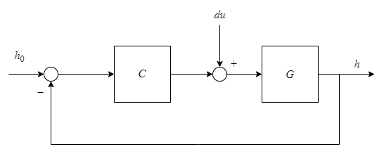
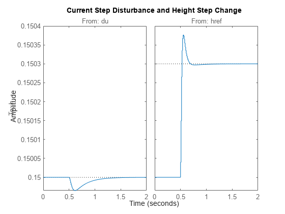
Compute and plot the step response of an LPV (lpvss) model. This example simulates the closed-loop step response of a levitating ball model defined in fcnMaglev.m to a disturbance du.

maglev-feedback.png

Create the model and discretize it.

hmin = 0.05; 
hmax = 0.25;
h0 = (hmin+hmax)/2;
Ts = 0.01;
Glpv = lpvss("h",@fcnMaglev,0,0,h0);
Glpvd = c2d(Glpv,Ts,"tustin"); 

Sample the LPV model for three height values and tune a PID controller.

hpid = linspace(hmin,hmax,3);
[Ga,Goffset] = sample(Glpvd,[],hpid);
wc = 50;
Ka = pidtune(Ga,"pidf",wc);
Ka.Tf = 0.01;

Create the gain-scheduled PID controller.

Ka.SamplingGrid = struct("h",hpid);
Koffset = struct("y",{Goffset.u});
Clpv = ssInterpolant(ss(Ka),Koffset);

Create the closed-loop model.

CL = feedback(Glpvd*[1,Clpv],1,2,1);
CL.InputName = {'du';'href'};
CL.OutputName = "h";

Get steady-state current for h = h0 to compute an appropriate size for the step disturbance at the plant input.

[~,~,~,~,~,~,~,u0] = Glpv.DataFunction(0,h0);

Compute and plot the response to the input disturbance and step change in reference. Set the baseline input signals du = 0 and h = h0 to specify the starting steady-state condition.

t = 0:Ts:2;
pFcn = @(k,x,u) x(1);
Config = RespConfig( ...
    Bias=[0;h0], ...
    Amplitude=0.2*[u0;h0]*Ts, ...
    Delay=0.5, ...
    InitialParameter=h0);
step(CL,t,pFcn,Config)
title("Current Step Disturbance and Height Step Change")

MATLAB figure

Input Arguments

collapse all

Dynamic system, specified as a SISO or MIMO dynamic system model or array of dynamic system models. Dynamic systems that you can use include:

  • Continuous-time or discrete-time numeric LTI models, such as tf, zpk, or ss models.

  • Generalized or uncertain LTI models such as genss or uss models. (Using uncertain models requires Robust Control Toolbox™ software.)

    • For tunable control design blocks, the function evaluates the model at its current value for both plotting and returning response data.

    • For uncertain control design blocks, the function plots the nominal value and random samples of the model. When you use output arguments, the function returns response data for the nominal model only.

  • Sparse state-space models such as sparss and mechss models.

  • Identified LTI models, such as idtf, idss, or idproc models. For such models, the function can also plot confidence intervals and return standard deviations of the frequency response. See Step Responses of Identified Models with Confidence Regions. (Using identified models requires System Identification Toolbox software.)

  • Linear time-varying (ltvss) and linear parameter-varying (lpvss) models.

This function does not support frequency-response data models such as frd, genfrd, or idfrd models.

If sys is an array of models, the function plots the responses of all models in the array on the same axes. See Step Response of Systems in a Model Array.

Time steps at which to compute the response, specified as one of the following:

  • Positive scalar tFinal— Compute the response from t = 0 to t = tFinal.

  • Two-element vector [t0 tFinal] — Compute the response from t = t0 to t = tFinal. (since R2023b)

  • Vector Ti:dt:Tf— Compute the response for the time points specified in t.

    • For continuous-time systems, dt is the sample time of a discrete approximation to the continuous system.

    • For discrete-time systems with a specified sample time, dt must match the sample time property Ts of sys.

    • For discrete-time systems with an unspecified sample time (Ts = -1), dt must be 1.

  • [] — Automatically select time values based on system dynamics.

When you specify a time range using either tFinal or [t0 tFinal]:

  • For continuous-time systems, the function automatically determines the size of the time step and number of points based on the system dynamics.

  • For discrete-time systems with a specified sample time, the function uses the sample time of sys as the step size.

  • For discrete-time systems with unspecified sample time (Ts = -1), the function interprets tFinal as the number of sampling periods to simulate with a sample time of 1 second.

Express t using the time units specified in the TimeUnit property of sys.

If you specified a step delay td using config, the function applies the step at t = t0+td.

Parameter trajectory of the LPV model, specified as a matrix or a function handle.

  • For exogenous or explicit trajectories, specify p as a matrix with dimensions N-by-Np, where N is the number of time samples and Np is the number of parameters.

    Thus, the row vector p(i,:) contains the parameter values at the ith time step.

  • For endogenous or implicit trajectories, specify p as a function handle of the form p = F(t,x,u) in continuous time and p = F(k,x,u) in discrete time that gives parameters as a function of time t or time sample k, state x, and input u.

    This option is useful when you want to simulate quasi-LPV models. For an example, see Step Response of LPV Model.

Configuration of the applied signal, specified as a RespConfig object. By default, step applies an input that goes from 0 to 1 at time t = 0. Use this input argument to change the configuration of the step input. See Response to Custom Step Input for an example.

For lpvss and ltvss models with offsets (x0(t),u0(t)), you can use RespConfig to define the input relative to u0(t,p) and initialize the simulation with the state x0(t,p).

Output Arguments

collapse all

Step response data, returned as an array.

  • For SISO systems, y is a column vector of the same length as t (if provided) or tOut (if you do not provide t).

  • For single-input, multi-output systems, y is a matrix with as many rows as there are time samples and as many columns as there are outputs. Thus, the jth column of y, or y(:,j), contains the step response of from the input to the jth output.

  • For MIMO systems, the step responses of each input channel are stacked up along the third dimension of y. The dimensions of y are then N-by-Ny-by-Nu, where:

    • N is the number of time samples.

    • Ny is the number of system outputs.

    • Nu is the number of system inputs.

    Thus, y(:,i,j) is a column vector containing the step response from the jth input to the ith output at the times specified in t or tOut.

Times at which step response is computed, returned as a vector. When you do not provide a specific vector t of times, step chooses this time vector based on the system dynamics. The times are expressed in the time units of sys.

State trajectories, returned as an array. When sys is a state-space model, x contains the evolution of the states of sys at each time in t or tOut. The dimensions of x are N-by-Nx-by-Nu, where:

  • N is the number of time samples.

  • Nx is the number of states.

  • Nu is the number of system inputs.

Thus, the evolution of the states in response to a step injected at the kth input is given by the array x(:,:,k). The row vector x(i,:,k) contains the state values at the ith time step.

Standard deviation of the step response of an identified model, returned as an array of the same dimensions as y. If sys does not contain parameter covariance information, then ysd is empty.

Parameter trajectories, returned as an array. When sys is a linear-parameter varying model, pOut contains the evolution of the parameters of sys at each time in t or tOut. The dimensions of pOut are N-by-Np-by-Nu, where:

  • N is the number of time samples.

  • Np is the number of parameters.

  • Nu is the number of system inputs.

Thus, the evolution of the parameters in response to a step injected at the kth input is given by the array pOut(:,:,k). The row vector pOut(i,:,k) contains the parameter values at the ith time step.

Tips

  • To simulate system responses to arbitrary input signals, use lsim.

Algorithms

To obtain samples of continuous-time models without internal delays, step converts such models to state-space models and discretizes them using a zero-order hold on the inputs. step chooses the sampling time for this discretization automatically based on the system dynamics, except when you supply the input time vector t in the form t = T0:dt:Tf. In that case, step uses dt as the sampling time. The resulting simulation time steps tOut are equisampled with spacing dt.

For systems with internal delays, Control System Toolbox™ software uses variable step solvers. As a result, the time steps tOut are not equisampled.

References

[1] L.F. Shampine and P. Gahinet, "Delay-differential-algebraic equations in control theory," Applied Numerical Mathematics, Vol. 56, Issues 3–4, pp. 574–588.
Version History

Introduced before R2006a

expand all