Linear System Analyzer
Analyze time-domain and frequency-domain responses of linear time-invariant (LTI) systems
Description
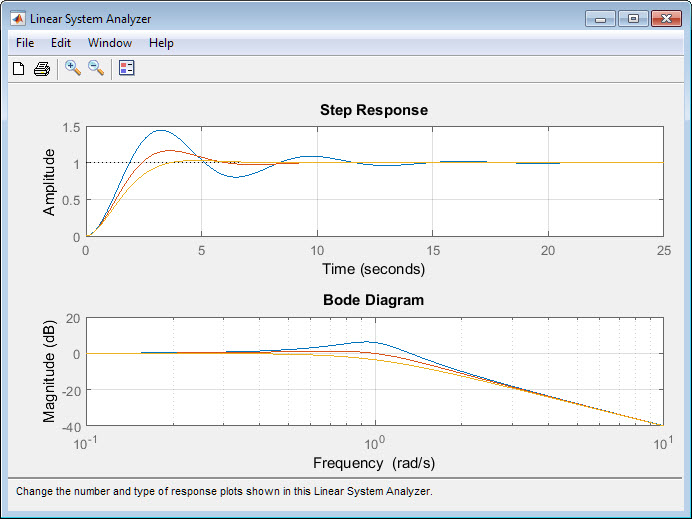
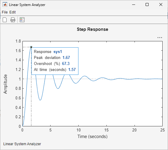
The Linear System Analyzer app lets you analyze time-domain and frequency-domain responses of LTI systems.
Using this app, you can:
View and compare the response plots of SISO and MIMO systems or of several linear models at the same time.
Generate time response plots such as step, impulse, and time response to arbitrary inputs.
Generate frequency response plots such as Bode, Nyquist, Nichols, singular-value, and pole-zero plots.
Inspect key response characteristics, such as rise time, maximum overshoot, and stability margins.
Linear System Analyzer can generate the following response plots:
Step response
Impulse response
Simulated time response to specified input signal
Simulated time response from specified initial conditions (state-space models only)
Bode diagram (magnitude and phase, or magnitude alone)
Nyquist plot
Nichols plot
Singular value plot
Pole/zero map and I/O pole/zero map
Open the Linear System Analyzer App
MATLAB® Toolstrip: On the Apps tab, under Control System Design and Analysis, click the app icon.
MATLAB command prompt: Enter
linearSystemAnalyzer.
Examples
To import models into Linear System Analyzer, select File > Import. The Import System Data dialog box opens.
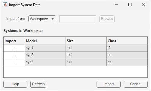
Under Import from, select whether to import a model from:
The MATLAB workspace by selecting
WorkspaceA MAT-file by selecting
MAT-file
In the Import column of the table, select one or models to import.
Click the Import.
To export models from Linear System Analyzer, select File > Export. The Linear System Analyzer Export dialog box opens.
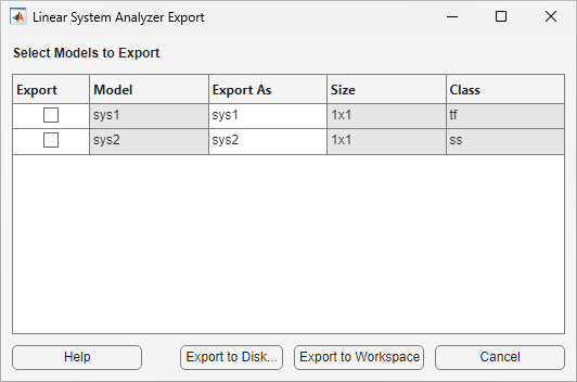
In the Export column of the table, select one or models to import.
To export models to the MATLAB workspace, click Export to Workspace.
To export models to a MAT-file, click Export to Disk.
In the Select File to Write dialog box, specify the name and location for saved MAT-file and click Save.
To remove models from Linear System Analyzer, select Edit > Delete Systems. The Linear System Analyzer Delete dialog box opens.
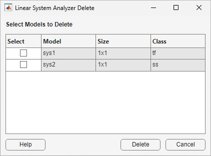
In the Select column, select one or models to delete.
Click Delete.
To interactively specify the types of responses to plot, in Linear System Analyzer, select Edit > Plot Configurations. The Plot Configurations dialog box opens.
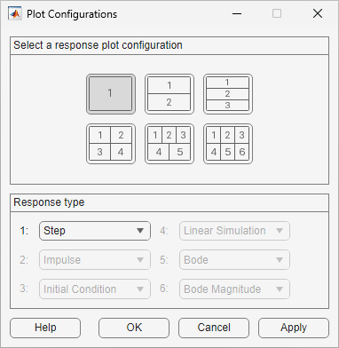
In the Select a response plot configuration section, select how many plots to show.
In the Response type section, use the drop-down lists to select the response type for each plot.
To update the plot configuration and close the dialog box, click OK.
To update the plot configuration without closing the dialog box, click Apply.
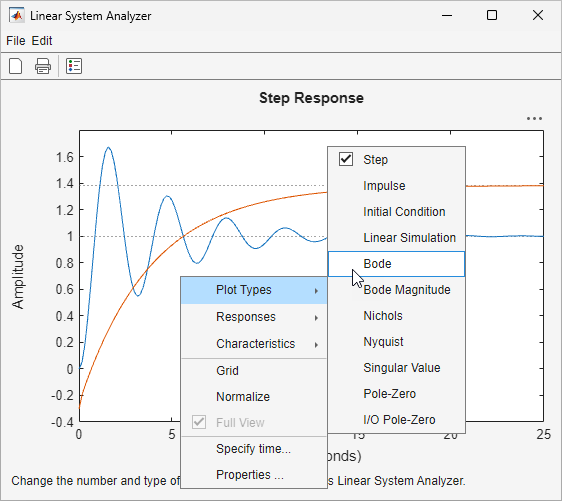
To switch the response type for an existing plot, right click the plot and, under Plot Types, select the type of response.
To interactively specify the line styles for responses, in Linear System Analyzer, select Edit > Response Styles. The Response Styles dialog box opens.
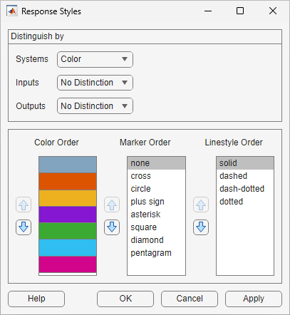
In the Distinguish by section, you can select how to distinguish between system, inputs, and outputs using the corresponding drop-down lists.
The selections in these drop-down lists are mutually exclusive, that is, you must use a different type of ordering for systems, inputs, and outputs.
Linear System Analyzer assigns response color, marker style, and line style based on the order specified under Color Order, Marker Order, and Linestyle Order, respectively.
You can modify these orders by clicking an item in the list and adjusting its position using the corresponding arrows.
To update the response styles and close the dialog box, click OK.
To update the response styles without closing the dialog box, click Apply.
To display response characteristics in a response plot, right-click the plot area and, under Characteristics, select a characteristic to display. You can display multiple characteristics on the same plot.
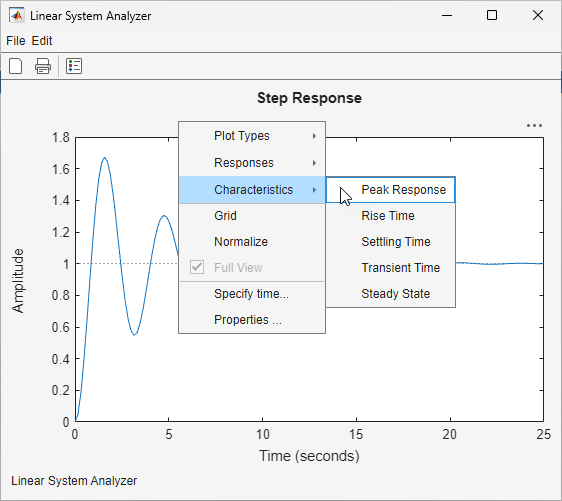
The available characteristics depend on the type of response plot.
| Response Plot | Available Characteristics |
|---|---|
| Step plot |
|
| Impulse plot |
|
| Initial condition plot | |
| Linear simulation plot | Peak response |
| Singular-value plot | |
| Bode plot |
|
| Nyquist plot | |
| Nichols plot | |
| Pole-zero plot | None |
| Pole/zero plot of each input/output pair |
The plot shows each characteristic using a marker on the response. To view information about the characteristic, click the marker.
Related Examples
Programmatic Use
linearSystemAnalyzer
opens the Linear System Analyzer app with no LTI
systems to analyze. For information on how to import a
system, see Import Models.
linearSystemAnalyzer(sys1,sys2,...,sysN)
opens Linear System Analyzer and displays the
step response of one or more dynamic system
models, sys1,
sys2, ...,
sysn. Such models include:
Numeric LTI models such as
tf,zpk, orssmodels.Identified models such as
idtf,idss, oridproc(requires System Identification Toolbox™ software).Generalized LTI models such as
genssorussmodels. For generalized LTI models without uncertainty, Linear System Analyzer plots the response of the nominal value of the model. For generalized models with uncertainty, the app plots the responses of 20 random samples of the uncertain system. (Uncertain models require Robust Control Toolbox™ software.)
linearSystemAnalyzer(sys1,LineSpec1,...,sysN,LineSpecN)
specifies the line style, marker, and color of each response
plot.
For more information about line style specifications, see the
LineSpec input argument of
the lsimplot function.
linearSystemAnalyzer(plottype,___)
opens Linear System Analyzer and displays the
response types specified by plottype.
You can use this syntax with any of the previous input
argument combinations. The plottype
argument can be any one of the following:
"step"— Step response"impulse"— Impulse response"lsim"— Linear simulation plot. If you do not specify input and time vectors using theextrassyntax, then the Linear Simulation Tool dialog box opens and prompts you to specify the input and time vectors."initial"— Initial condition plot (state-space models only). You must specify an initial condition using use theextrassyntax."bode"— Bode diagram"bodemag"— Bode magnitude diagram"nyquist"— Nyquist plot"nichols"— Nichols plot"sigma"— Singular value plot"pzmap"— Pole/zero map"iopzmap"— Pole/zero map of each input/output pair of the LTI system
To open Linear System Analyzer with multiple response
plots, specify string array of up to six plot types. For
example, the following command opens the app with a step
response and a Nyquist plot for system
sys.
linearSystemAnalyzer(["step","nyquist"],sys)
linearSystemAnalyzer(plottype,sys1,sys2,...,sysn,extras)
specifies additional input arguments specific to the type of
response plot. extras can be one or
more of the input arguments available for the function
corresponding to the plot type, except the
plotoptions argument and
name-value arguments.
To determine appropriate arguments for
extras, see the reference
pages of the functions corresponding to each plot type, such
as stepplot, bodeplot, or initialplot.
For example, suppose plottype is
"step". Then,
extras enables you to use the
additional arguments that you could use with the stepplot command, such as the desired
final time, Tfinal. Thus, the following
command opens the app with a step response plot of
sys, with a final time of
Tfinal.
linearSystemAnalyzer("step",sys,Tfinal)
If plottype is
"initial", you must use
extras to supply initial
conditions IC. For example, the
following command sets the initial condition to vector
x0 of state values.
linearSystemAnalyzer("initial",sys,x0)
If plottype is "lsim",
you can use extras to specify input
vector u and time vector
t.
h = linearSystemAnalyzer(___)
returns a handle to the Linear System
Analyzer figure. You can use this syntax
with any of the previous combinations of input
arguments. Use the handle to modify previously
opened Linear System Analyzer
instances, as described in the next two
syntaxes.
linearSystemAnalyzer("clear",h)
clears the plots and data from the Linear System
Analyzer session corresponding to handle
h. To clear multiple app
instances at once, set h to a vector of
handles.
linearSystemAnalyzer("current",sys1,sys2,...,sysn,h)
adds the responses of the systems sys1,
sys2, ...,
sysn to the Linear
System Analyzer session corresponding to
handle h. To update multiple app
instances at once, set h to a vector of
handles. If the new systems have different I/O dimensions
from the currently displayed systems, the app clears the
existing responses and displays only the new ones.
Version History
Introduced in R2015a
See Also
Apps
Functions
stepplot|impulseplot|lsimplot|initialplot|iopzplot|pzplot|bodeplot|bodemag|nyquistplot|nicholsplot|sigmaplot
MATLAB Command
You clicked a link that corresponds to this MATLAB command:
Run the command by entering it in the MATLAB Command Window. Web browsers do not support MATLAB commands.
Select a Web Site
Choose a web site to get translated content where available and see local events and offers. Based on your location, we recommend that you select: .
You can also select a web site from the following list
How to Get Best Site Performance
Select the China site (in Chinese or English) for best site performance. Other MathWorks country sites are not optimized for visits from your location.
Americas
- América Latina (Español)
- Canada (English)
- United States (English)
Europe
- Belgium (English)
- Denmark (English)
- Deutschland (Deutsch)
- España (Español)
- Finland (English)
- France (Français)
- Ireland (English)
- Italia (Italiano)
- Luxembourg (English)
- Netherlands (English)
- Norway (English)
- Österreich (Deutsch)
- Portugal (English)
- Sweden (English)
- Switzerland
- United Kingdom (English)