Main Content

stepinfo

Rise time, settling time, and other step-response characteristics

Description

stepinfo lets you compute step-response characteristics for a dynamic system model or for an array of step-response data. For a step response y(t), stepinfo computes characteristics relative to yinit and yfinal, where yinit is the initial offset, that is, the value before the step is applied, and yfinal is the steady-state value of the response. These values depend on the syntax you use.

  • For a dynamic system model sys, stepinfo uses yinit = 0 and yfinal = steady-state value.

  • For an array of step-response data [y,t], stepinfo uses yinit = 0 and yfinal = last sample value of y, unless you explicitly specify these values.

For more information on how stepinfo computes the step-response characteristics, see Algorithms.

The following figure illustrates some of the characteristics stepinfo computes for a step response. For this response, assume that y(t) = 0 for t < 0, so yinit = 0.
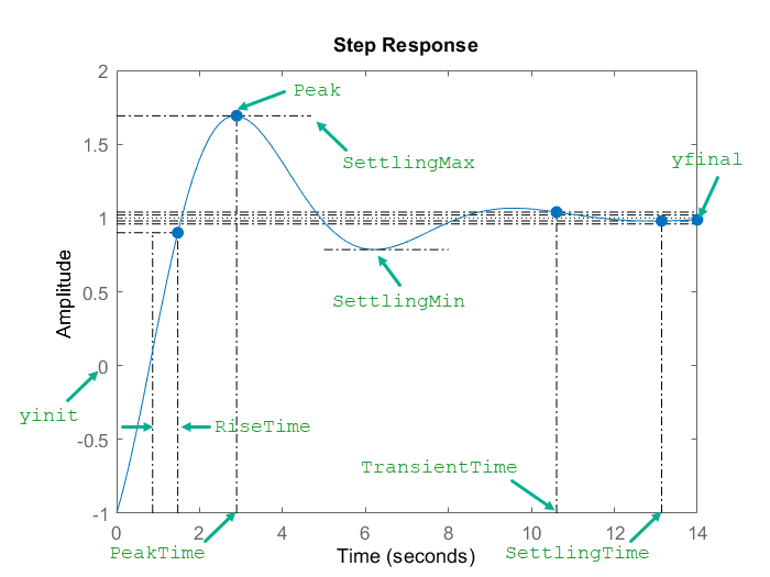
Step response characteristics. The figure shows peak response, peak time, rise time, settling time, and transient time of the response.

S = stepinfo(sys) computes the step-response characteristics for a dynamic system model sys. This syntax uses yinit = 0 and yfinal = steady-state value for computing the characteristics that depend on these values.

example

S = stepinfo(y,t) computes step-response characteristics from an array of step-response data y and a corresponding time vector t. For SISO system responses, y is a vector with the same number of entries as t. For MIMO response data, y is an array containing the responses of each I/O channel. This syntax uses yinit = 0 and the last value in y (or the last value in each channel's corresponding response data) as yfinal.

S = stepinfo(y,t,yfinal) computes step-response characteristics relative to the steady-state value yfinal. This syntax is useful when you know that the expected steady-state system response differs from the last value in y for reasons such as measurement noise. This syntax uses yinit = 0.

For SISO responses, t and y are vectors with the same length NS. For systems with NU inputs and NY outputs, you can specify y as an NS-by-NY-by-NU array (see step) and yfinal as an NY-by-NU array. stepinfo then returns a NY-by-NU structure array S of response characteristics corresponding to each I/O pair.

example

S = stepinfo(y,t,yfinal,yinit) computes step-response characteristics relative to the response initial value yinit. This syntax is useful when your y data has an initial offset; that is, y is nonzero before the step occurs.

For SISO responses, t and y are vectors with the same length NS. For systems with NU inputs and NY outputs, you can specify y as an NS-by-NY-by-NU array and yinit as an NY-by-NU array. stepinfo then returns a NY-by-NU structure array S of response characteristics corresponding to each I/O pair.

example

S = stepinfo(___,'SettlingTimeThreshold',ST) lets you specify the threshold ST used in the definition of settling and transient times. The default value is ST = 0.02 (2%). You can use this syntax with any of the previous input-argument combinations.

example

S = stepinfo(___,'RiseTimeLimits',RT) lets you specify the lower and upper thresholds used in the definition of rise time. By default, the rise time is the time the response takes to rise from 10% to 90% of the way from the initial value to the steady-state value (RT = [0.1 0.9]). The upper threshold RT(2) is also used to calculate SettlingMin and SettlingMax. These values are the minimum and maximum values of the response occurring after the response reaches the upper threshold. You can use this syntax with any of the previous input-argument combinations.

example

Examples

collapse all

Compute step-response characteristics, such as rise time, settling time, and overshoot, for a dynamic system model. For this example, use a continuous-time transfer function:

sys=s2+5s+5s4+1.65s3+5s2+6.5s+2.

Create the transfer function and examine its step response.

sys = tf([1 5 5],[1 1.65 5 6.5 2]);
step(sys)

MATLAB figure

The plot shows that the response rises in a few seconds, and then rings down to a steady-state value of about 2.5. Compute the characteristics of this response using stepinfo.

S = stepinfo(sys)
S = struct with fields:
         RiseTime: 3.8456
    TransientTime: 27.9762
     SettlingTime: 27.9762
      SettlingMin: 2.0689
      SettlingMax: 2.6873
        Overshoot: 7.4915
       Undershoot: 0
             Peak: 2.6873
         PeakTime: 8.0530

Here, the function uses yinit= 0 to compute characteristics for the dynamic system model sys.

By default, the settling time is the time it takes for the error to stay below 2% of |yinit-yfinal|. The result S.SettlingTime shows that for sys, this condition occurs after about 28 seconds. The default definition of rise time is the time it takes for the response to go from 10% to 90% of the way from yinit= 0 to yfinal. S.RiseTime shows that for sys, this rise occurs in less than 4 seconds. The maximum overshoot is returned in S.Overshoot. For this system, the peak value S.Peak, which occurs at the time S.PeakTime, overshoots by about 7.5% of the steady-state value.

For a MIMO system, stepinfo returns a structure array in which each entry contains the response characteristics of the corresponding I/O channel of the system. For this example, use a two-output, two-input discrete-time system. Compute the step-response characteristics.

A = [0.68 -0.34; 0.34 0.68];
B = [0.18 -0.05; 0.04 0.11];
C = [0 -1.53; -1.12 -1.10];
D = [0 0; 0.06 -0.37];
sys = ss(A,B,C,D,0.2);

S = stepinfo(sys)
S=2×2 struct array with fields:
    RiseTime
    TransientTime
    SettlingTime
    SettlingMin
    SettlingMax
    Overshoot
    Undershoot
    Peak
    PeakTime

Access the response characteristics for a particular I/0 channel by indexing into S. For instance, examine the response characteristics for the response from the first input to the second output of sys, corresponding to S(2,1).

S(2,1)
ans = struct with fields:
         RiseTime: 0.4000
    TransientTime: 2.8000
     SettlingTime: 3
      SettlingMin: -0.6724
      SettlingMax: -0.5188
        Overshoot: 24.6476
       Undershoot: 11.1224
             Peak: 0.6724
         PeakTime: 1

To access a particular value, use dot notation. For instance, extract the rise time of the (2,1) channel.

rt21 = S(2,1).RiseTime
rt21 = 
0.4000

You can use SettlingTimeThreshold and RiseTimeThreshold to change the default percentage for settling and rise times, respectively, as described in the Algorithms section. For this example, use the system given by:

sys=s2+5s+5s4+1.65s3+6.5s+2.

Create the transfer function.

sys = tf([1 5 5],[1 1.65 5 6.5 2]);

Compute the time it takes for the error in the response of sys to stay below 0.5% of the gap |yfinal-yinit|. To do so, set SettlingTimeThreshold to 0.5%, or 0.005.

S1 = stepinfo(sys,SettlingTimeThreshold=0.005);
st1 = S1.SettlingTime
st1 = 
46.1325

Compute the time it takes the response of sys to rise from 5% to 95% of the way from yinit to yfinal. To do so, set RiseTimeThreshold to a vector containing those bounds.

S2 = stepinfo(sys,RiseTimeThreshold=[0.05 0.95]);
rt2 = S2.RiseTime
rt2 = 
4.1690

You can define percentages for both settling time and rise time in the same computation.

S3 = stepinfo(sys,...
    SettlingTimeThreshold=0.005, ...
    RiseTimeThreshold=[0.05 0.95])
S3 = struct with fields:
         RiseTime: 4.1690
    TransientTime: 46.1325
     SettlingTime: 46.1325
      SettlingMin: 2.0689
      SettlingMax: 2.6873
        Overshoot: 7.4915
       Undershoot: 0
             Peak: 2.6873
         PeakTime: 8.0530

You can extract step-response characteristics from step-response data even if you do not have a model of your system. For instance, suppose you have measured the response of your system to a step input and saved the resulting response data in a vector y of response values at the times stored in another vector t. Load the response data and examine it.

load StepInfoData t y
plot(t,y)

Figure contains an axes object. The axes object contains an object of type line.

Compute step-response characteristics from this response data using stepinfo. If you do not specify the steady-state response value yfinal, then stepinfo assumes that the last value in the response vector y is the steady-state response. Because the data has some noise, the last value in y is likely not the true steady-state response value. When you know what the steady-state value should be, you can provide it to stepinfo. For this example, suppose that the steady-state response is 2.4.

S1 = stepinfo(y,t,2.4)
S1 = struct with fields:
         RiseTime: 1.2897
    TransientTime: 19.6478
     SettlingTime: 19.6439
      SettlingMin: 2.0219
      SettlingMax: 3.3302
        Overshoot: 38.7575
       Undershoot: 0
             Peak: 3.3302
         PeakTime: 3.4000

Because of the noise in the data, the default definition of the settling time is too stringent, resulting in an arbitrary value of almost 20 seconds. To allow for the noise, increase the settling-time threshold from the default 2% to 5%.

S2 = stepinfo(y,t,2.4,'SettlingTimeThreshold',0.05)
S2 = struct with fields:
         RiseTime: 1.2897
    TransientTime: 10.4201
     SettlingTime: 10.4149
      SettlingMin: 2.0219
      SettlingMax: 3.3302
        Overshoot: 38.7575
       Undershoot: 0
             Peak: 3.3302
         PeakTime: 3.4000

Settling time and transient time are equal when the peak error emax is equal to the gap |yfinal-yinit| (see Algorithms), which is the case for models with no undershoot or feedthrough and with less than 100% overshoot. They tend to differ for models with feedthrough, zeros at the origin, unstable zeros (undershoot), or large overshoot.

Consider the following models.

  • sys1 — System with direct feedthrough

  • sys2 — System with zero at origin

  • sys3 — Nonminimum phase system with undershoot

  • sys4 — System with large overshoot

s = tf("s");
sys1 = 1+tf(1,[1 1]);
sys2 = tf([1 0],[1 1]);
sys3 = tf([-3 1],[1 2 1]);
sys4 = (s/0.5 + 1)/(s^2 + 0.2*s + 1);

step(sys1,sys2,sys3,sys4)
grid on
legend("Feedthrough", ...
    "Zero at origin", ...
    "Nonminimum phase with undershoot", ...
    "Large overshoot")

MATLAB figure

Compute the step-response characteristics.

S1 = stepinfo(sys1)
S1 = struct with fields:
         RiseTime: 1.6095
    TransientTime: 3.9121
     SettlingTime: 3.2190
      SettlingMin: 1.8005
      SettlingMax: 1.9993
        Overshoot: 0
       Undershoot: 0
             Peak: 1.9993
         PeakTime: 7.3222

S2 = stepinfo(sys2)
S2 = struct with fields:
         RiseTime: 0
    TransientTime: 3.9121
     SettlingTime: NaN
      SettlingMin: 6.6069e-04
      SettlingMax: 1
        Overshoot: Inf
       Undershoot: 0
             Peak: 1
         PeakTime: 0

S3 = stepinfo(sys3)
S3 = struct with fields:
         RiseTime: 2.9198
    TransientTime: 6.5839
     SettlingTime: 7.3229
      SettlingMin: 0.9004
      SettlingMax: 0.9991
        Overshoot: 0
       Undershoot: 88.9466
             Peak: 0.9991
         PeakTime: 10.7900

S4 = stepinfo(sys4)
S4 = struct with fields:
         RiseTime: 0.3896
    TransientTime: 40.3317
     SettlingTime: 46.5052
      SettlingMin: -0.2796
      SettlingMax: 2.7571
        Overshoot: 175.7137
       Undershoot: 27.9629
             Peak: 2.7571
         PeakTime: 1.8850

Examine the plots and characteristics. For these models, the settling time and transient time differ because the peak error exceeds the gap between the initial and the final value. For models such as sys2, the settling time is returned as NaN because the steady-state value is zero.

In this example, you compute the step-response characteristics from step-response data that has an initial offset. This means that the value of the response data is nonzero before the step occurs.

Load the step-response data and examine the plot.

load stepDataOffset.mat
plot(stepOffset.Time,stepOffset.Data)

Figure contains an axes object. The axes object contains an object of type line.

If you do not specify yfinal and yinit, then stepinfo assumes that yfinal is the last value in the response vector y and yinit is zero. When you know what the steady-state and initial values are, you can provide them to stepinfo. Here, the steady state of the response yfinal is 0.9 and the initial offset yinit is 0.2.

Compute step-response characteristics from this response data.

S = stepinfo(stepOffset.Data,stepOffset.Time,0.9,0.2)
S = struct with fields:
         RiseTime: 0.0084
    TransientTime: 1.0662
     SettlingTime: 1.0662
      SettlingMin: 0.8461
      SettlingMax: 1.0878
        Overshoot: 26.8259
       Undershoot: 0.0429
             Peak: 0.8878
         PeakTime: 1.0225

Here, the peak value of this response is 0.8878 because stepinfo measures the maximum deviation from yinit.

Input Arguments

collapse all

Dynamic system, specified as a SISO or MIMO dynamic system model. Dynamic systems that you can use include:

  • Continuous-time or discrete-time numeric LTI models, such as tf, zpk, or ss models.

  • Generalized or uncertain LTI models such as genss or uss (Robust Control Toolbox) models. (Using uncertain models requires Robust Control Toolbox™ software.) For generalized models, stepinfo computes the step-response characteristics using the current value of tunable blocks and the nominal value of uncertain blocks.

  • Identified LTI models, such as idtf (System Identification Toolbox), idss (System Identification Toolbox), or idproc (System Identification Toolbox) models. (Using identified models requires System Identification Toolbox™ software.)

Step-response data, specified as one of the following:

  • For SISO response data, a vector of length Ns, where Ns is the number of samples in the response data

  • For MIMO response data, an Ns-by-Ny-by-Nu array, where Ny is the number of system outputs and Nu is the number of system inputs

Time vector corresponding to the response data in y, specified as a vector of length Ns.

Steady-state value, specified as a scalar or an array.

  • For SISO response data, specify a scalar value.

  • For MIMO response data, specify an Ny-by-Nu array, where each entry provides the steady-state response value for the corresponding system channel.

If you do not provide yfinal, then stepinfo uses the last value in the corresponding channel of y as the steady-state response value.

This argument is only supported when you provide step-response data as an input. For a dynamic system model sys as an input, stepinfo uses yfinal = steady-state value to compute the characteristics that depend on this value.

Value of y before the step occurs, specified as a scalar or an array.

  • For SISO response data, specify a scalar value.

  • For MIMO response data, specify an Ny-by-Nu array, where each entry provides the response initial value for the corresponding system channel.

If you do not provide yinit, then stepinfo uses zero as the response initial value.

The response y(0) at t = 0 is equal to yinit for systems without feedthrough. However, the two quantities differ in the presence of feedthrough because of the discontinuity at t = 0.

For example, the following figure shows the step response of a system with feedthrough sys = tf([-1 0.2 1],[1 0.7 1]).

Step response of a system with feedthrough equal to negative1

Here, yinit is zero and the feedthrough value is –1.

This argument is only supported when you provide step-response data as an input. For a dynamic system model sys as an input, stepinfo uses yinit = 0 to compute the characteristics that depend on this value.

Threshold for defining settling and transient times, specified as a scalar value between 0 and 1. To change the default settling and transient time definitions (see Algorithms), set ST to a different value. For instance, to measure when the error falls below 5%, set ST to 0.05.

Threshold for defining rise time, specified as a 2-element row vector of nondescending values between 0 and 1. To change the default rise time definition (see Algorithms), set RT to a different value. For instance, to define the rise time as the time it takes for the response to rise from 5% to 95% from the initial value to the steady-state value, set RT to [0.05 0.95].

Output Arguments

collapse all

Step-response characteristics, returned as a structure containing the fields:

  • RiseTime

  • TransientTime

  • SettlingTime

  • SettlingMin

  • SettlingMax

  • Overshoot

  • Undershoot

  • Peak

  • PeakTime

For more information on how stepinfo defines these characteristics, see Algorithms.

For MIMO models or responses data, S is a structure array in which each entry contains the step-response characteristics of the corresponding I/O channel. For instance, if you provide a 3-input, 3-output model or an array of response data, then S(2,3) contains the characteristics of the response from the third input to the second output. For an example, see Step-Response Characteristics of MIMO System.

If sys is unstable, then all step-response characteristics are NaN, except for Peak and PeakTime, which are Inf.

Algorithms

For a step response y(t), stepinfo computes characteristics relative to yinit and yfinal. By default, for a dynamic system model sys, stepinfo uses yinit = 0 and yfinal = steady-state value.

This table shows how stepinfo computes each characteristic.

Step-Response CharacteristicDescription
RiseTimeTime it takes for the response to rise from 10% to 90% of the way from yinit to yfinal
TransientTime

The first time T such that the error |y(t) – yfinal| ≤ SettlingTimeThreshold × emax for tT, where emax is the maximum error |y(t) – yfinal| for t ≥ 0.

By default, SettlingTimeThreshold = 0.02 (2% of the peak error). Transient time measures how quickly the transient dynamics die off.

SettlingTime

The first time T such that the error |y(t) – yfinal| ≤ SettlingTimeThreshold × |yfinalyinit| for tT.

By default, SettlingTime measures the time it takes for the error to stay below 2% of |yfinalyinit|.

SettlingMinMinimum value of y(t) once the response has risen
SettlingMaxMaximum value of y(t) once the response has risen
OvershootPercentage overshoot. Relative to the normalized response ynorm(t) = (y(t) – yinit)/(yfinalyinit), the overshoot is the larger of zero and 100 × max(ynorm(t) – 1).
UndershootPercentage undershoot. Relative to the normalized response ynorm(t), the undershoot is the smaller of zero and –100 × min(ynorm(t) ).
PeakPeak value of |y(t) – yinit|
PeakTimeTime at which the peak value occurs

Version History

Introduced in R2006a

expand all

See Also

|