connect
Block diagram interconnections of dynamic systems
Syntax
Description
sysc = connect(sys1,...sysN,inputs,outputs)sys1,...sysN
based on signal names. The connect command interconnects the block
diagram elements by connecting input and output channels with matching names, as specified
in the InputName and OutputName properties of
sys1,...,sysN. The aggregate model sysc is a
dynamic system model with inputs and outputs specified by inputs and
outputs, respectively.
sysc = connect(sys1,...sysN,inputs,outputs,APs)AnalysisPoint at every signal location
specified in APs. Use analysis points to mark locations of interest
which are internal signals in the aggregate model. For instance, a location at which you
want to extract a loop transfer function or measure the stability margins is a location of
interest.
sysc = connect(blksys,connections,inputs,outputs)sysc out of an aggregate,
unconnected model blksys. The matrix connections
specifies how the outputs and inputs of blksys interconnect. For
index-based interconnections, inputs and outputs
are index vectors that specify which inputs and outputs of blksys are
the external inputs and outputs of sysc. This syntax can be convenient
when you do not want to assign names to all inputs and outputs of all models to connect.
However, in general, it is easier to keep track of named signals.
sysc = connect(___,opts)sysc. To create
opts, use connectOptions. You can use
opts with the input arguments of any of the previous syntaxes.
Examples
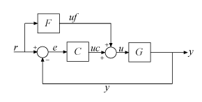
Create an aggregate model of the following block diagram from r to y.

This model contains a plant G, a feedback controller C, and a feedforward controller F. Create dynamic system models representing each of these elements.
C = pid(2,1);
G = zpk([],[-1,-1,-5],1);
F = tf(3,[1 3]);
In preparation for building the block diagram using signal names, assign to each element the input and output names shown in the block diagram. To do so, set the InputName and OutputName properties of the elements.
C.InputName = "e";
C.OutputName = "uc";

G.InputName = "u";
G.OutputName = "y";

F.InputName = "r";
F.OutputName = "uf";
The block diagram also contains two summing junctions. One summing junction takes the difference between the reference signal r and the plant output y to compute the error signal e. The other summing junction adds the feedforward controller output uf to the feedback controller output uc to compute the plant input u. Use the sumblk command to create these summing junctions. To use sumblk, write the expression for the summing junction as a string.
S1 = sumblk("e = r - y");
S2 = sumblk("u = uc + uf");
sumblk returns a tf model object representing the sum, with the input names and output names you provide in the expression. For instance, examine the signal names of S1.
S1
S1 =

  From input "r" to output "e":
  1

  From input "y" to output "e":
  -1

Static gain.
Model Properties
You can now combine all the elements to create an aggregate model representing the response of the system in the block diagram from r to y. Provide connect with the list of elements to combine, the desired input signal of the aggregate model r, and the desired output signal y. The connect command automatically joins the elements by connecting inputs and outputs with matching names.
T = connect(G,C,F,S1,S2,"r","y");
size(T)
State-space model with 1 outputs, 1 inputs, and 5 states.
T.InputName
ans = 1×1 cell array
    {'r'}
T.OutputName
ans = 1×1 cell array
    {'y'}
Create the control system of the previous example, where G, C, and F are all two-input, two-output models.
In this example, the signals r, y, e, and so on are all vector signals of two elements each. First, create the models and name their inputs and outputs.
C = [pid(2,1), 0;
     0,pid(5,6)];
F = [tf(3,[1 3]), 0;
     0, tf(3,[1 3])];
G = ss(-1,[1,2],[1;-1],0);
Assign the input and output names.
C.InputName = "e";
C.OutputName = "uc";

G.InputName = "u";
G.OutputName = "y";

F.InputName = "r";
F.OutputName = "uf";
When you assign single names to vector-valued signals, the software automatically applies vector expansion to give each input and output channel a unique name. For instance, examine the names of the plant inputs.
G.InputName
ans = 2×1 cell
    {'u(1)'}
    {'u(2)'}
This example uses vector expansion for the signal names of all MIMO components of the block diagram. You can instead name the signals individually, provided that you match the names of signals you want to join. For an example that uses individually named signals for some block-diagram elements, see MIMO Control System with Fixed and Tunable Components.
Next, create the vector-valued summing junction. sumblk also automatically expands the signal names you provide in the sum expression for the vector signals, as you can verify by examining the input names of S2.
S1 = sumblk("e = r - y",2);
S2 = sumblk("u = uc + uf",2);
S2.InputName
ans = 4×1 cell
    {'uc(1)'}
    {'uc(2)'}
    {'uf(1)'}
    {'uf(2)'}
Combine all the elements to create an aggregate model representing the response r to y, that is, from [r(1),r(2)] to [y(1),y(2)].
T = connect(G,C,F,S1,S2,"r","y");
size(T)
State-space model with 2 outputs, 2 inputs, and 5 states.
T.InputName
ans = 2×1 cell
    {'r(1)'}
    {'r(2)'}
T.OutputName
ans = 2×1 cell
    {'y(1)'}
    {'y(2)'}
Consider the following block diagram.
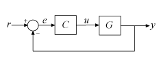
You can create a model of this closed-loop system using feedback and use the model to study the system response from r to y. Suppose that you also want to study the response of the closed-loop system to a disturbance injected at the plant input. To do so, you can use connect to build the system, inserting an analysis point at the location u.
First create plant and controller models, naming the inputs and outputs as shown in the diagram.
C = pid(2,1);
C.InputName = "e";
C.OutputName = "u";

G = zpk([],[-1,-1],1);
G.InputName = "u";
G.OutputName = "y";
Create a summing junction that takes the difference between the reference signal r and the plant output y to compute the error signal e.
Sum = sumblk("e = r - y");Combine C, G, and the summing junction to create the aggregate model. Use the APs input argument to connect to insert an analysis point at u.
input = "r";
output = "y";
APs = "u";
CL = connect(G,C,Sum,input,output,APs)
Generalized continuous-time state-space model with 1 outputs, 1 inputs, 3 states, and the following blocks:
  CONNECT_AP1: Analysis point, 1 channels, 1 occurrences.
Model Properties

Type "ss(CL)" to see the current value and "CL.Blocks" to interact with the blocks.
This closed-loop model is a generalized state-space (genss) model containing an AnalysisPoint control design block. To see the name of the analysis point channel in CL, use getPoints.
getPoints(CL)
ans = 1×1 cell array
    {'u'}
Inserting the analysis point creates a model that is equivalent to the following block diagram, where AP_u designates the AnalysisPoint block with channel name u.

Use the analysis point to extract system responses. For example, the following commands extract the open-loop transfer at u and the closed-loop response at y to a disturbance injected at u.
L = getLoopTransfer(CL,"u",-1);
CLdist = getIOTransfer(CL,"u","y");
You can use index-based interconnection to connect model elements without naming all their inputs and outputs. To see how, create a model of the following feedback loop from r to y using index-based interconnection.

First, create the plant and controller, the elements of the closed-loop system.
C = pid(2,1);
G = zpk([],[-1,-1,-5],1);
Use append to group the elements into a single, unconnected aggregate model.
blksys = append(C,G);
append arranges the specified models into a MIMO stacked model, as shown in the following diagram.

To make this stacked model equivalent to the feedback loop, connect must make the following connections:
The input of
Greceives the output ofC, orw1feeds intou2.The input of
Creceives the negative of the output ofG, or-w2feeds into-u1.
To instruct connect to make these connections, construct a matrix in which each row specifies one connection or summing junction in terms of the input vector u and output vector y of blksys.
connections = [2  1;  %  w1 feeds into u2
               1 -2]; % -w2 feeds into u1
Finally, specify by index which inputs and outputs of blksys to use for the external inputs and outputs of the closed-loop model.
inputs = 1;  % r drives u1
outputs = 2; % y is y2
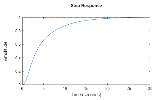
You can now complete the closed-loop model.
sysc = connect(blksys,connections,inputs,outputs);
step(sysc)
This example shows what to expect when combining two models created with connect, each containing analysis points.
Create a model of cascaded feedback loops using these commands.
G1 = tf([1],[1 0]);
G1.u = 'OuterError';
G1.y = 'InnerCmd';
G2 = tf([1], [1 1]);
G2.u = 'InnerError';
G2.y = 'ActuatorCmd';
SumOuter = sumblk('OuterError = OuterCmd - Outer');
SumInner = sumblk('InnerError = InnerCmd - Inner');
Sys1 = connect(G1,G2,SumOuter,SumInner,{'OuterCmd','Outer','Inner'},'ActuatorCmd', {'InnerError','OuterError'})
Generalized continuous-time state-space model with 1 outputs, 3 inputs, 2 states, and the following blocks:
  CONNECT_AP1: Analysis point, 2 channels, 1 occurrences.
Model Properties

Type "ss(Sys1)" to see the current value and "Sys1.Blocks" to interact with the blocks.
The generalized model Sys1 contains a single analysis point block with channels InnerError and OuterError.
Alternatively, you can define inner and outer loops separately.
P1 = connect(G1,SumOuter,{'OuterCmd','Outer'},'InnerCmd','OuterError')Generalized continuous-time state-space model with 1 outputs, 2 inputs, 1 states, and the following blocks: CONNECT_AP1: Analysis point, 1 channels, 1 occurrences. Model Properties Type "ss(P1)" to see the current value and "P1.Blocks" to interact with the blocks.
P2 = connect(G2,SumInner,{'InnerCmd','Inner'},'ActuatorCmd','InnerError')Generalized continuous-time state-space model with 1 outputs, 2 inputs, 1 states, and the following blocks: CONNECT_AP1: Analysis point, 1 channels, 1 occurrences. Model Properties Type "ss(P2)" to see the current value and "P2.Blocks" to interact with the blocks.
Both P1 and P2 have an analysis block named CONNECT_AP1. Now combine these two models to create a model Sys2 of the cascaded loop.
Sys2 = connect(P1,P2,{'OuterCmd','Outer','Inner'},'ActuatorCmd')Generalized continuous-time state-space model with 1 outputs, 3 inputs, 2 states, and the following blocks: CONNECT_AP1: Analysis point, 1 channels, 1 occurrences. CONNECT_AP2: Analysis point, 1 channels, 1 occurrences. Model Properties Type "ss(Sys2)" to see the current value and "Sys2.Blocks" to interact with the blocks.
This model contains two separate analysis point blocks with names CONNECT_AP1 and CONNECT_AP2. The AnalysisPoint blocks of P1 and P2 are automatically renamed to avoid conflict.