modelCalibrationPlot

Scatter plot of predicted and observed LGDs

Since R2023a

Syntax

modelCalibrationPlot(lgdModel,data)

modelCalibrationPlot(___,Name,Value)

h = modelCalibrationPlot(ax,___,Name,Value)

Description

modelCalibrationPlot(lgdModel,data) returns a scatter plot of observed vs. predicted loss given default (LGD) data with a linear fit. modelCalibrationPlot supports comparison against a reference model. By default, modelCalibrationPlot plots in the LGD scale.

modelCalibrationPlot(___,Name,Value) specifies options using one or more name-value pair arguments in addition to the input arguments in the previous syntax. You can use the ModelLevel name-value pair argument to compute metrics using the underlying model's transformed scale.

h = modelCalibrationPlot(ax,___,Name,Value) specifies options using one or more name-value pair arguments in addition to the input arguments in the previous syntax and returns the figure handle h.

Examples

Generate a Scatter Plot of Predicted and Observed LGDs Using Regression LGD Model

This example shows how to use fitLGDModel to fit data with a Regression model and then use modelCalibrationPlot to generate a scatter plot for predicted and observed LGDs.

Load Data

Load the loss given default data.

load LGDData.mat
head(data)

      LTV        Age         Type           LGD   
    _______    _______    ___________    _________

    0.89101    0.39716    residential     0.032659
    0.70176     2.0939    residential      0.43564
    0.72078     2.7948    residential    0.0064766
    0.37013      1.237    residential     0.007947
    0.36492     2.5818    residential            0
      0.796     1.5957    residential      0.14572
    0.60203     1.1599    residential     0.025688
    0.92005    0.50253    investment      0.063182

Partition Data

Separate the data into training and test partitions.

rng('default'); % for reproducibility
NumObs = height(data);

c = cvpartition(NumObs,'HoldOut',0.4);
TrainingInd = training(c);
TestInd = test(c);

Create Regression LGD Model

Use fitLGDModel to create a Regression model using training data.

lgdModel = fitLGDModel(data(TrainingInd,:),'regression');
disp(lgdModel)    

  Regression with properties:

    ResponseTransform: "logit"
    BoundaryTolerance: 1.0000e-05
              ModelID: "Regression"
          Description: ""
      UnderlyingModel: [1x1 classreg.regr.CompactLinearModel]
        PredictorVars: ["LTV"    "Age"    "Type"]
          ResponseVar: "LGD"
           WeightsVar: ""

Display the underlying model.

lgdModel.UnderlyingModel

ans = 
Compact linear regression model:
    LGD_logit ~ 1 + LTV + Age + Type

Estimated Coefficients:
                       Estimate       SE        tStat       pValue  
                       ________    ________    _______    __________

    (Intercept)        -4.7549      0.36041    -13.193    3.0997e-38
    LTV                 2.8565      0.41777     6.8377    1.0531e-11
    Age                -1.5397     0.085716    -17.963    3.3172e-67
    Type_investment     1.4358       0.2475     5.8012     7.587e-09


Number of observations: 2093, Error degrees of freedom: 2089
Root Mean Squared Error: 4.24
R-squared: 0.206,  Adjusted R-Squared: 0.205
F-statistic vs. constant model: 181, p-value = 2.42e-104

Generate Scatter Plot of Predicted and Observed LGDs

Use modelCalibrationPlot to generate a scatter plot of predicted and observed LGDs for the test data set. The ModelLevel name-value pair argument modifies the output only for Regression models, not Tobit models, because there are no response transformations for the Tobit model.

modelCalibrationPlot(lgdModel,data(TestInd,:),ModelLevel="underlying")

Generate Scatter Plot of Predicted and Observed LGDs Using Tobit LGD Model

This example shows how to use fitLGDModel to fit data with a Tobit model and then use modelCalibrationPlot to generate a scatter plot of predicted and observed LGDs.

Load Data

Load the loss given default data.

load LGDData.mat
head(data)

      LTV        Age         Type           LGD   
    _______    _______    ___________    _________

    0.89101    0.39716    residential     0.032659
    0.70176     2.0939    residential      0.43564
    0.72078     2.7948    residential    0.0064766
    0.37013      1.237    residential     0.007947
    0.36492     2.5818    residential            0
      0.796     1.5957    residential      0.14572
    0.60203     1.1599    residential     0.025688
    0.92005    0.50253    investment      0.063182

Partition Data

Separate the data into training and test partitions.

rng('default'); % for reproducibility
NumObs = height(data);

c = cvpartition(NumObs,'HoldOut',0.4);
TrainingInd = training(c);
TestInd = test(c);

Create Tobit LGD Model

Use fitLGDModel to create a Tobit model using training data.

lgdModel = fitLGDModel(data(TrainingInd,:),'tobit');
disp(lgdModel)    

  Tobit with properties:

      CensoringSide: "both"
          LeftLimit: 0
         RightLimit: 1
            Weights: [0x1 double]
            ModelID: "Tobit"
        Description: ""
    UnderlyingModel: [1x1 risk.internal.credit.TobitModel]
      PredictorVars: ["LTV"    "Age"    "Type"]
        ResponseVar: "LGD"
         WeightsVar: ""

Display the underlying model.

disp(lgdModel.UnderlyingModel)

Tobit regression model:
     LGD = max(0,min(Y*,1))
     Y* ~ 1 + LTV + Age + Type

Estimated coefficients:
                       Estimate        SE         tStat       pValue  
                       _________    _________    _______    __________

    (Intercept)         0.058257     0.027277     2.1357      0.032819
    LTV                  0.20126     0.031352     6.4193    1.6887e-10
    Age                -0.095407    0.0072648    -13.133             0
    Type_investment      0.10208     0.018077     5.6471    1.8544e-08
    (Sigma)              0.29288    0.0057081     51.309             0

Number of observations: 2093
Number of left-censored observations: 547
Number of uncensored observations: 1521
Number of right-censored observations: 25
Log-likelihood: -698.383

Generate Scatter Plot of Predicted and Observed LGDs

Use modelCalibrationPlot to generate a scatter plot of predicted and observed LGDs for the test data set.

modelCalibrationPlot(lgdModel,data(TestInd,:))

Generate Scatter Plot of Predicted and Observed LGDs Using Beta LGD Model

This example shows how to use fitLGDModel to fit data with a Beta model and then use modelCalibrationPlot to generate a scatter plot of predicted and observed LGDs.

Load Data

Load the loss given default data.

load LGDData.mat
head(data)

      LTV        Age         Type           LGD   
    _______    _______    ___________    _________

    0.89101    0.39716    residential     0.032659
    0.70176     2.0939    residential      0.43564
    0.72078     2.7948    residential    0.0064766
    0.37013      1.237    residential     0.007947
    0.36492     2.5818    residential            0
      0.796     1.5957    residential      0.14572
    0.60203     1.1599    residential     0.025688
    0.92005    0.50253    investment      0.063182

Partition Data

Separate the data into training and test partitions.

rng('default'); % for reproducibility
NumObs = height(data);

c = cvpartition(NumObs,'HoldOut',0.4);
TrainingInd = training(c);
TestInd = test(c);

Create Beta LGD Model

Use fitLGDModel to create a Beta model using training data.

lgdModel = fitLGDModel(data(TrainingInd,:),'Beta');
disp(lgdModel)    

  Beta with properties:

    BoundaryTolerance: 1.0000e-05
              ModelID: "Beta"
          Description: ""
      UnderlyingModel: [1x1 risk.internal.credit.BetaModel]
        PredictorVars: ["LTV"    "Age"    "Type"]
          ResponseVar: "LGD"
           WeightsVar: ""

Display the underlying model.

disp(lgdModel.UnderlyingModel)

Beta regression model:
     logit(LGD) ~ 1_mu + LTV_mu + Age_mu + Type_mu
     log(LGD) ~ 1_phi + LTV_phi + Age_phi + Type_phi

Estimated coefficients:
                           Estimate       SE        tStat       pValue  
                           ________    ________    _______    __________

    (Intercept)_mu          -1.3772     0.13201    -10.433             0
    LTV_mu                   0.6027     0.15087     3.9948    6.6993e-05
    Age_mu                 -0.47464    0.040264    -11.788             0
    Type_investment_mu      0.45372    0.085143     5.3289    1.0941e-07
    (Intercept)_phi        -0.16336     0.12591    -1.2974       0.19462
    LTV_phi                0.055886     0.14719    0.37969       0.70421
    Age_phi                 0.22887    0.040335     5.6743     1.586e-08
    Type_investment_phi    -0.14102    0.078155    -1.8044      0.071313

Number of observations: 2093
Log-likelihood: -5291.04

Generate Scatter Plot of Predicted and Observed LGDs

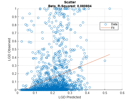
Use modelCalibrationPlot to generate a scatter plot of predicted and observed LGDs for the test data set.

modelCalibrationPlot(lgdModel,data(TestInd,:))

Visualize Calibration for Residuals or Other Variables

modelCalibrationPlot generates a scatter plot of observed vs. predicted LGD values. The 'XData' and 'YData' name-value arguments allow you to visualize the residuals or generate a scatter plot against a variable of interest.

Load Data

Load the loss given default data.

load LGDData.mat
head(data)

      LTV        Age         Type           LGD   
    _______    _______    ___________    _________

    0.89101    0.39716    residential     0.032659
    0.70176     2.0939    residential      0.43564
    0.72078     2.7948    residential    0.0064766
    0.37013      1.237    residential     0.007947
    0.36492     2.5818    residential            0
      0.796     1.5957    residential      0.14572
    0.60203     1.1599    residential     0.025688
    0.92005    0.50253    investment      0.063182

Partition Data

Separate the data into training and test partitions.

rng('default'); % for reproducibility
NumObs = height(data);

c = cvpartition(NumObs,'HoldOut',0.4);
TrainingInd = training(c);
TestInd = test(c);

Create Regression LGD Model

Use fitLGDModel to create a Regression model using training data.

lgdModel = fitLGDModel(data(TrainingInd,:),'regression');
disp(lgdModel)

  Regression with properties:

    ResponseTransform: "logit"
    BoundaryTolerance: 1.0000e-05
              ModelID: "Regression"
          Description: ""
      UnderlyingModel: [1x1 classreg.regr.CompactLinearModel]
        PredictorVars: ["LTV"    "Age"    "Type"]
          ResponseVar: "LGD"
           WeightsVar: ""

Display the underlying model.

disp(lgdModel.UnderlyingModel)

Compact linear regression model:
    LGD_logit ~ 1 + LTV + Age + Type

Estimated Coefficients:
                       Estimate       SE        tStat       pValue  
                       ________    ________    _______    __________

    (Intercept)        -4.7549      0.36041    -13.193    3.0997e-38
    LTV                 2.8565      0.41777     6.8377    1.0531e-11
    Age                -1.5397     0.085716    -17.963    3.3172e-67
    Type_investment     1.4358       0.2475     5.8012     7.587e-09


Number of observations: 2093, Error degrees of freedom: 2089
Root Mean Squared Error: 4.24
R-squared: 0.206,  Adjusted R-Squared: 0.205
F-statistic vs. constant model: 181, p-value = 2.42e-104

Generate Scatter Plot of Predicted and Observed LGDs

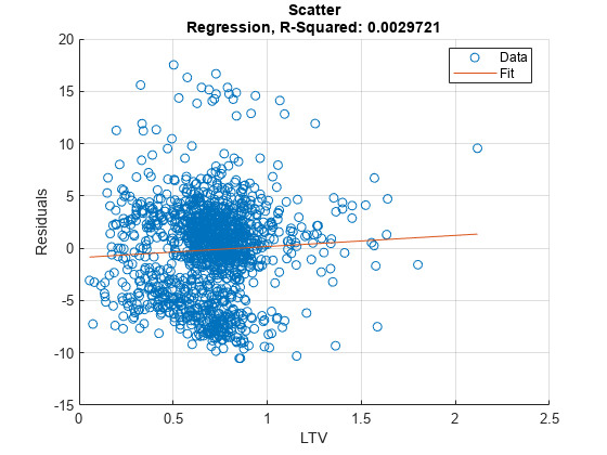
Use modelCalibrationPlot to generate a scatter plot of residuals against LTV values.

modelCalibrationPlot(lgdModel,data(TestInd,:),XData='LTV',YData='residuals')

For Regression models, the 'ModelLevel' name-value argument allows you to visualize the plot using the underlying model scale.

modelCalibrationPlot(lgdModel,data(TestInd,:),XData='LTV',YData='residuals',ModelLevel='underlying')

For categorical variables, modelCalibrationPlot uses a swarm chart. For more information, see swarmchart.

modelCalibrationPlot(lgdModel,data(TestInd,:),XData='Type',YData='residuals',ModelLevel='underlying')

Input Arguments

lgdModel — Loss given default model

Regression object | Tobit object

Loss given default model, specified as a previously created Regression, Tobit, or Beta object using fitLGDModel.

Data Types: object

data — Data

table

Data, specified as a NumRows-by-NumCols table with predictor and response values. The variable names and data types must be consistent with the underlying model.

Data Types: table

ax — Valid axis object

object

(Optional) Valid axis object, specified as an ax object that is created using axes. The plot will be created in the axes specified by the optional ax argument instead of in the current axes (gca). The optional argument ax must precede any of the input argument combinations.

Data Types: object

Name-Value Arguments

Specify optional pairs of arguments as Name1=Value1,...,NameN=ValueN, where Name is the argument name and Value is the corresponding value. Name-value arguments must appear after other arguments, but the order of the pairs does not matter.

Example: modelCalibrationPlot(lgdModel,data(TestInd,:),DataID='Testing',YData=residuals,XData='LTV')

DataID — Data set identifier

"" (default) | character vector | string

Data set identifier, specified as DataID and a character vector or string. The DataID is included in the output for reporting purposes.

Data Types: char | string

ModelLevel — Model level

'top' (default) | character vector with value 'top' or 'underlying' | string with value "top" or "underlying"

Model level, specified as ModelLevel and a character vector or string.

• 'top' — The accuracy metrics are computed in the LGD scale at the top model level.

• 'underlying' — For a Regression model only, the metrics are computed in the underlying model's transformed scale. The metrics are computed on the transformed LGD data.

Note

ModelLevel has no effect for a Tobit or Beta model because there is no response transformation.

Data Types: char | string

ReferenceLGD — LGD values predicted for data by reference model

[ ] (default) | numeric vector

LGD values predicted for data by the reference model, specified as ReferenceLGD and a NumRows-by-1 numeric vector. The scatter plot output is plotted for both the lgdModel object and the reference model.

Data Types: double

ReferenceID — Identifier for the reference model

'Reference' (default) | character vector | string

Identifier for the reference model, specified as ReferenceID and a character vector or string. 'ReferenceID' is used in the scatter plot output for reporting purposes.

Data Types: char | string

XData — Data to plot on x-axis

'predicted' (default) | character vector with value 'predicted', 'observed', 'residuals', or VariableName | string with value | "predicted", "observed", "residuals", or VariableName

Data to plot on x-axis, specified as XData and a character vector or string for one of the following:

• 'predicted' — Plot the predicted LGD values in the x-axis.

• 'observed' — Plot the observed LGD values in the x-axis.

• 'residuals' — Plot the residuals in the x-axis.

• VariableName — Use the name of the variable in the data input, not necessarily a model variable, to plot in the x-axis.

Data Types: char | string

YData — Data to plot on y-axis

'predicted' (default) | character vector with value 'predicted', 'observed', or 'residuals' | string with value | "predicted", "observed", or "residuals"

Data to plot on y-axis, specified as YData and a character vector or string for one of the following:

• 'predicted' — Plot the predicted LGD values in the y-axis.

• 'observed' — Plot the observed LGD values in the y-axis.

• 'residuals' — Plot the residuals in the y-axis.

Data Types: char | string

Output Arguments

h — Figure handle

handle object

Figure handle for the scatter and line objects, returned as handle object.

More About

Model Calibration Plot

The modelCalibrationPlot function returns a scatter plot of observed vs. predicted loss given default (LGD) data with a linear fit and reports the R-square of the linear fit.

The XData name-value pair argument allows you to change the x values on the plot. By default, predicted LGD values are plotted in the x-axis, but predicted LGD values, residuals, or any variable in the data input, not necessarily a model variable, can be used as x values. If the selected XData is a categorical variable, a swarm chart is used. For more information, see swarmchart.

The YData name-value pair argument allows users to change the y values on the plot. By default, observed LGD values are plotted in the y-axis, but predicted LGD values or residuals can also be used as y values. YData does not support table variables.

For Regression models, if ModelLevel is set to 'underlying', the LGD data is transformed into the underlying model's scale. The transformed data is shown on the plot. The ModelLevel name-value pair argument has no effect for Tobit models.

The linear fit and reported R-squared value always correspond to the linear regression model with the plotted y values as response and the plotted x values as the only predictor.

References

[1] Baesens, Bart, Daniel Roesch, and Harald Scheule. Credit Risk Analytics: Measurement Techniques, Applications, and Examples in SAS. Wiley, 2016.

[2] Bellini, Tiziano. IFRS 9 and CECL Credit Risk Modelling and Validation: A Practical Guide with Examples Worked in R and SAS. San Diego, CA: Elsevier, 2019.

Version History

Introduced in R2023a