modelDiscrimination

Compute AUROC and ROC data

Since R2021a

Syntax

DiscMeasure = modelDiscrimination(lgdModel,data)

[DiscMeasure,DiscData] = modelDiscrimination(___,Name,Value)

Description

DiscMeasure = modelDiscrimination(lgdModel,data) computes the area under the receiver operating characteristic curve (AUROC). modelDiscrimination supports segmentation and comparison against a reference model and also alternative methods to discretize the LGD response into a binary variable.

[DiscMeasure,DiscData] = modelDiscrimination(___,Name,Value) specifies options using one or more name-value pair arguments in addition to the input arguments in the previous syntax.

Examples

Compute AUROC and ROC Using a Regression LGD Model

This example shows how to use fitLGDModel to fit data with a Regression model and then use modelDiscrimination to compute AUROC and ROC.

Load Data

Load the loss given default data.

load LGDData.mat
head(data)

      LTV        Age         Type           LGD   
    _______    _______    ___________    _________

    0.89101    0.39716    residential     0.032659
    0.70176     2.0939    residential      0.43564
    0.72078     2.7948    residential    0.0064766
    0.37013      1.237    residential     0.007947
    0.36492     2.5818    residential            0
      0.796     1.5957    residential      0.14572
    0.60203     1.1599    residential     0.025688
    0.92005    0.50253    investment      0.063182

Partition Data

Separate the data into training and test partitions.

rng('default'); % for reproducibility
NumObs = height(data);

c = cvpartition(NumObs,'HoldOut',0.4);
TrainingInd = training(c);
TestInd = test(c);

Create a Regression LGD Model

Use fitLGDModel to create a Regression model using training data. You can also use fitLGDModel to create a Tobit model by changing the lgdModel input argument to 'Tobit'.

lgdModel = fitLGDModel(data(TrainingInd,:),'Regression');
disp(lgdModel)    

  Regression with properties:

    ResponseTransform: "logit"
    BoundaryTolerance: 1.0000e-05
              ModelID: "Regression"
          Description: ""
      UnderlyingModel: [1×1 classreg.regr.CompactLinearModel]
        PredictorVars: ["LTV"    "Age"    "Type"]
          ResponseVar: "LGD"
           WeightsVar: ""

Display the underlying model.

disp(lgdModel.UnderlyingModel)

Compact linear regression model:
    LGD_logit ~ 1 + LTV + Age + Type

Estimated Coefficients:
                       Estimate       SE        tStat       pValue  
                       ________    ________    _______    __________

    (Intercept)        -4.7549      0.36041    -13.193    3.0997e-38
    LTV                 2.8565      0.41777     6.8377    1.0531e-11
    Age                -1.5397     0.085716    -17.963    3.3172e-67
    Type_investment     1.4358       0.2475     5.8012     7.587e-09


Number of observations: 2093, Error degrees of freedom: 2089
Root Mean Squared Error: 4.24
R-squared: 0.206,  Adjusted R-Squared: 0.205
F-statistic vs. constant model: 181, p-value = 2.42e-104

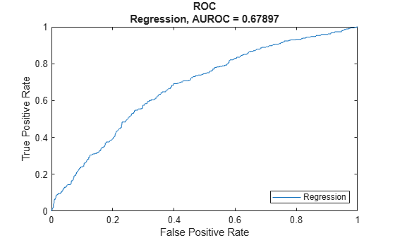
Compute AUROC and ROC Data

Use modelDiscrimination to compute the AUROC and ROC for the test data set.

[DiscMeasure,DiscData] = modelDiscrimination(lgdModel,data(TestInd,:),'ShowDetails',true)

DiscMeasure=1×4 table
                   AUROC      Segment      SegmentCount    WeightedCount
                  _______    __________    ____________    _____________

    Regression    0.67897    "all_data"        1394            1394     

DiscData=1395×3 table
        X             Y           T   
    __________    _________    _______

             0            0    0.87604
             0    0.0029326    0.87604
             0    0.0058651     0.7515
    0.00094967    0.0058651    0.44074
     0.0018993    0.0058651    0.43569
     0.0018993    0.0087977    0.40058
      0.002849    0.0087977    0.31703
      0.002849      0.01173    0.30375
      0.002849     0.014663    0.28789
      0.002849     0.017595    0.27996
     0.0037987     0.017595    0.27026
     0.0047483     0.017595    0.26868
      0.005698     0.017595    0.26854
      0.005698     0.020528    0.26682
     0.0066477     0.020528    0.26668
     0.0066477      0.02346    0.24923
      ⋮

You can visualize the ROC data using modelDiscriminationPlot.

modelDiscriminationPlot(lgdModel,data(TestInd,:))

Compute AUROC and ROC Using Tobit LGD Model

This example shows how to use fitLGDModel to fit data with a Tobit model and then use modelDiscrimination to compute AUROC and ROC.

Load Data

Load the loss given default data.

load LGDData.mat
head(data)

      LTV        Age         Type           LGD   
    _______    _______    ___________    _________

    0.89101    0.39716    residential     0.032659
    0.70176     2.0939    residential      0.43564
    0.72078     2.7948    residential    0.0064766
    0.37013      1.237    residential     0.007947
    0.36492     2.5818    residential            0
      0.796     1.5957    residential      0.14572
    0.60203     1.1599    residential     0.025688
    0.92005    0.50253    investment      0.063182

Partition Data

Separate the data into training and test partitions.

rng('default'); % for reproducibility
NumObs = height(data);

c = cvpartition(NumObs,'HoldOut',0.4);
TrainingInd = training(c);
TestInd = test(c);

Create a Tobit LGD Model

Use fitLGDModel to create a Tobit model using training data.

lgdModel = fitLGDModel(data(TrainingInd,:),'tobit');
disp(lgdModel)    

  Tobit with properties:

      CensoringSide: "both"
          LeftLimit: 0
         RightLimit: 1
            Weights: [0×1 double]
            ModelID: "Tobit"
        Description: ""
    UnderlyingModel: [1×1 risk.internal.credit.TobitModel]
      PredictorVars: ["LTV"    "Age"    "Type"]
        ResponseVar: "LGD"
         WeightsVar: ""

Display the underlying model.

disp(lgdModel.UnderlyingModel)

Tobit regression model:
     LGD = max(0,min(Y*,1))
     Y* ~ 1 + LTV + Age + Type

Estimated coefficients:
                       Estimate        SE         tStat       pValue  
                       _________    _________    _______    __________

    (Intercept)         0.058257     0.027279     2.1356       0.03283
    LTV                  0.20126      0.03136     6.4177    1.7064e-10
    Age                -0.095407    0.0072633    -13.135             0
    Type_investment      0.10208     0.018077     5.6471    1.8542e-08
    (Sigma)              0.29288    0.0057084     51.306             0

Number of observations: 2093
Number of left-censored observations: 547
Number of uncensored observations: 1521
Number of right-censored observations: 25
Log-likelihood: -698.383

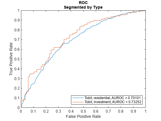
Compute AUROC and ROC Data

Use modelDiscrimination to compute the AUROC and ROC for the test data set.

DiscMeasure = modelDiscrimination(lgdModel,data(TestInd,:),'ShowDetails',true,'SegmentBy',"Type",'DiscretizeBy',"median")

DiscMeasure=2×4 table
                                AUROC        Segment       SegmentCount    WeightedCount
                               _______    _____________    ____________    _____________

    Tobit, Type=residential    0.70101    "residential"        1152            1152     
    Tobit, Type=investment     0.73252    "investment"          242             242     

You can visualize the ROC using modelDiscriminationPlot.

modelDiscriminationPlot(lgdModel,data(TestInd,:),'SegmentBy',"Type",'DiscretizeBy',"median")

Compute AUROC and ROC Using Beta LGD Model

This example shows how to use fitLGDModel to fit data with a Beta model and then use modelDiscrimination to compute AUROC and ROC.

Load Data

Load the loss given default data.

load LGDData.mat
head(data)

      LTV        Age         Type           LGD   
    _______    _______    ___________    _________

    0.89101    0.39716    residential     0.032659
    0.70176     2.0939    residential      0.43564
    0.72078     2.7948    residential    0.0064766
    0.37013      1.237    residential     0.007947
    0.36492     2.5818    residential            0
      0.796     1.5957    residential      0.14572
    0.60203     1.1599    residential     0.025688
    0.92005    0.50253    investment      0.063182

Partition Data

Separate the data into training and test partitions.

rng('default'); % for reproducibility
NumObs = height(data);

c = cvpartition(NumObs,'HoldOut',0.4);
TrainingInd = training(c);
TestInd = test(c);

Create a Beta LGD Model

Use fitLGDModel to create a risk_ug#object_model_beta_lgd model using training data.

lgdModel = fitLGDModel(data(TrainingInd,:),'Beta');
disp(lgdModel)    

  Beta with properties:

    BoundaryTolerance: 1.0000e-05
              ModelID: "Beta"
          Description: ""
      UnderlyingModel: [1×1 risk.internal.credit.BetaModel]
        PredictorVars: ["LTV"    "Age"    "Type"]
          ResponseVar: "LGD"
           WeightsVar: ""

Display the underlying model.

disp(lgdModel.UnderlyingModel)

Beta regression model:
     logit(LGD) ~ 1_mu + LTV_mu + Age_mu + Type_mu
     log(LGD) ~ 1_phi + LTV_phi + Age_phi + Type_phi

Estimated coefficients:
                           Estimate       SE        tStat       pValue  
                           ________    ________    _______    __________

    (Intercept)_mu          -1.3772     0.13201    -10.433             0
    LTV_mu                  0.60269     0.15087     3.9947    6.7021e-05
    Age_mu                 -0.47464    0.040264    -11.788             0
    Type_investment_mu      0.45372    0.085143     5.3289    1.0941e-07
    (Intercept)_phi        -0.16336     0.12591    -1.2974       0.19465
    LTV_phi                0.055881     0.14719    0.37965       0.70424
    Age_phi                 0.22887    0.040335     5.6742    1.5867e-08
    Type_investment_phi    -0.14102    0.078155    -1.8044      0.071312

Number of observations: 2093
Log-likelihood: -5291.04

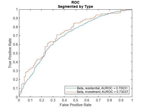
Compute AUROC and ROC Data

Use modelDiscrimination to compute the AUROC and ROC for the test data set.

DiscMeasure = modelDiscrimination(lgdModel,data(TestInd,:),'ShowDetails',true,'SegmentBy',"Type",'DiscretizeBy',"median")

DiscMeasure=2×4 table
                               AUROC        Segment       SegmentCount    WeightedCount
                              _______    _____________    ____________    _____________

    Beta, Type=residential    0.70031    "residential"        1152            1152     
    Beta, Type=investment     0.73037    "investment"          242             242     

You can visualize the ROC using modelDiscriminationPlot.

modelDiscriminationPlot(lgdModel,data(TestInd,:),'SegmentBy',"Type",'DiscretizeBy',"median")

Input Arguments

lgdModel — Loss given default model

Regression object | Tobit object | Beta object

Loss given default model, specified as a previously created Regression, Tobit, or Beta object using fitLGDModel.

Data Types: object

data — Data

table

Data, specified as a NumRows-by-NumCols table with predictor and response values. The variable names and data types must be consistent with the underlying model.

Data Types: table

Name-Value Arguments

Specify optional pairs of arguments as Name1=Value1,...,NameN=ValueN, where Name is the argument name and Value is the corresponding value. Name-value arguments must appear after other arguments, but the order of the pairs does not matter.

Before R2021a, use commas to separate each name and value, and enclose Name in quotes.

Example: [DiscMeasure,DiscData] = modelDiscrimination(lgdModel,data(TestInd,:),'DataID','Testing','DiscretizeBy','median')

DataID — Data set identifier

"" (default) | character vector | string

Data set identifier, specified as the comma-separated pair consisting of 'DataID' and a character vector or string. The DataID is included in the output for reporting purposes.

Data Types: char | string

DiscretizeBy — Discretization method for LGD data

'mean' (default) | character vector with value 'mean', 'median', 'positive', or 'total' | string with value "mean", "median", "positive", or "total"

Discretization method for LGD data, specified as the comma-separated pair consisting of 'DiscretizeBy' and a character vector or string.

• 'mean' — Discretized response is 1 if observed LGD is greater than or equal to the mean LGD, 0 otherwise.

• 'median' — Discretized response is 1 if observed LGD is greater than or equal to the median LGD, 0 otherwise.

• 'positive' — Discretized response is 1 if observed LGD is positive, 0 otherwise (full recovery).

• 'total' — Discretized response is 1 if observed LGD is greater than or equal to 1 (total loss), 0 otherwise.

Data Types: char | string

SegmentBy — Name of column in data input used to segment data set

"" (default) | character vector | string

Name of a column in the data input, not necessarily a model variable, to be used to segment the data set, specified as the comma-separated pair consisting of 'SegmentBy' and a character vector or string. One AUROC is reported for each segment, and the corresponding ROC data for each segment is returned in the optional output.

Data Types: char | string

ShowDetails — Indicates if output includes columns showing segment value and segment count

false (default) | logical

Since R2022a

Indicates if the output includes columns showing segment value and segment count, specified as the comma-separated pair consisting of 'ShowDetails' and a scalar logical.

Data Types: logical

ReferenceLGD — LGD values predicted for data by reference model

[] (default) | numeric vector

LGD values predicted for data by the reference model, specified as the comma-separated pair consisting of 'ReferenceLGD' and a NumRows-by-1 numeric vector. The modelDiscrimination output information is reported for both the lgdModel object and the reference model.

Data Types: double

ReferenceID — Identifier for the reference model

'Reference' (default) | character vector | string

Identifier for the reference model, specified as the comma-separated pair consisting of 'ReferenceID' and a character vector or string. 'ReferenceID' is used in the modelDiscrimination output for reporting purposes.

Data Types: char | string

Output Arguments

DiscMeasure — AUROC information for each model and each segment

table

AUROC information for each model and each segment, returned as a table. DiscMeasure has a single column named 'AUROC' and the number of rows depends on the number of segments and whether you use a ReferenceID for a reference model. The row names of DiscMeasure report the model IDs, segment, and data ID. If the optional ShowDetails name-value argument is true, the DiscMeasure output displays Segment, SegmentCount, and WeightedCount columns.

Note

If you do not specify SegmentBy and use ShowDetails to request the segment details, the two columns are added and show the Segment column as "all_data" and the sample size (minus missing values) for the SegmentCount column.

DiscData — ROC data for each model and each segment

table

ROC data for each model and each segment, returned as a table. There are three columns for the ROC data, with column names 'X', 'Y', and 'T', where the first two are the X and Y coordinates of the ROC curve, and T contains the corresponding thresholds. For more information, see Model Discrimination or perfcurve.

If you use SegmentBy, the function stacks the ROC data for all segments and DiscData has a column with the segmentation values to indicate where each segment starts and ends.

If reference model data is given, the DiscData outputs for the main and reference models are stacked, with an extra column 'ModelID' indicating where each model starts and ends.

More About

Model Discrimination

Model discrimination measures the risk ranking.

The modelDiscrimination function computes the area under the receiver operator characteristic (AUROC) curve, sometimes called simply the area under the curve (AUC). This metric is between 0 and 1 and higher values indicate better discrimination.

To compute the AUROC, you need a numeric prediction and a binary response. For loss given default (LGD) models, the predicted LGD is used directly as the prediction. However, the observed LGD must be discretized into a binary variable. By default, observed LGD values greater than or equal to the mean observed LGD are assigned a value of 1, and values below the mean are assigned a value of 0. This discretized response is interpreted as "high LGD" vs. "low LGD." Therefore, the modelDiscrimination function measures how well the predicted LGD separates the "high LGD" vs. the "low LGD" observations. You can change the discretization criterion with the DiscretizeBy name-value pair argument.

To plot the receiver operator characteristic (ROC) curve, use the modelDiscriminationPlot function. However, if the ROC curve data is needed, use the optional DiscData output argument from the modelDiscrimination function.

The ROC curve is a parametric curve that plots the proportion of

• High LGD cases with predicted LGD greater than or equal to a parameter t, or true positive rate (TPR)

• Low LGD cases with predicted LGD greater than or equal to the same parameter t, or false positive rate (FPR)

The parameter t sweeps through all the observed predicted LGD values for the given data. The DiscData optional output contains the TPR in the 'X' column, the FPR in the 'Y' column, and the corresponding parameters t in the 'T' column. For more information about ROC curves, see ROC Curve and Performance Metrics.

If the LGD model object is created by using the WeightsVar name-value argument, the AUROC and ROC are weighted quantities.

References

[1] Baesens, Bart, Daniel Roesch, and Harald Scheule. Credit Risk Analytics: Measurement Techniques, Applications, and Examples in SAS. Wiley, 2016.

[2] Bellini, Tiziano. IFRS 9 and CECL Credit Risk Modelling and Validation: A Practical Guide with Examples Worked in R and SAS. San Diego, CA: Elsevier, 2019.

Version History

Introduced in R2021a

R2024a: Support for WeightedCount column in DiscMeasure output

The DiscMeasure output supports an additional column for WeightedCount.

R2022b: Support for Beta model

The lgdModel input supports an option for a Beta model object that you can create using fitLGDModel.

R2022a: Additional option for ShowDetails

There is an additional name-value pair for ShowDetails to indicate if the DiscMeasure output includes columns for Segment value and the SegmentCount.