rfckt.cpw
Coplanar waveguide transmission line
Description
Use the rfckt.cpw object to create a coplanar waveguide
transmission line that is characterized by line dimensions, stub type, and
termination.
A coplanar waveguide transmission line is shown in cross-section in the following figure. Its physical characteristics include the conductor width (w), the conductor thickness (t), the slot width (s), the substrate height (d), and the permittivity constant (ε).

Note
txlineCPW is recommended over rfckt.cpw because
it enables you to:
Create a coplanar waveguide or conductor backed transmission line.
Build a
circuitobject with a coplanar waveguide or conductor backed transmission line.Input the
txlineCPWobject to thecoplanarWaveguideobject from RF PCB Toolbox™ for EM modeling.Model a coplanar waveguide or conductor backed element in an RF chain created using an
rfbudgetobject or the RF Budget Analyzer app, and then export this element to RF Blockset™ or torfsystemSystem object™ for circuit envelope analysis.
(since R2023b)
Creation
Description
h = rfckt.cpw returns a coplanar waveguide
transmission line object whose properties are set to their default
values.
h = rfckt.cpw(Name,Value) sets properties using one
or more name-value pairs. For example,
rfckt.cpw('ConductorWidth',0.3) creates an RF
coplanar waveguide transmission line with a width of 0.3 meters. You can
specify multiple name-value pairs. Enclose each property name in a quote.
Properties not specified retain their default values.
Properties
Object Functions
analyze | Analyze RFCKT object in frequency domain |
calculate | Calculate specified parameters for rfckt objects or rfdata objects |
circle | Draw circles on Smith Chart |
extract | Extract specified network parameters from rfckt object or data object |
listformat | List valid formats for specified circuit object parameter |
listparam | List valid parameters for specified circuit object |
loglog | Plot specified circuit object parameters using log-log scale |
plot | Plot circuit object parameters on X-Y plane |
plotyy | Plot parameters of RF circuit or RF data on xy-plane with two Y-axes |
getop | Display operating conditions |
polar | Plot specified object parameters on polar coordinates |
semilogx | Plot RF circuit object parameters using log scale for x-axis |
semilogy | Plot RF circuit object parameters using log scale for y-axis |
smith | Plot circuit object parameters on Smith Chart |
write | Write RF data from circuit or data object to file |
getz0 | Calculate characteristic impedance of RFCKT transmission line object |
read | Read RF data from file to new or existing circuit or data object |
restore | Restore data to original frequencies |
getop | Display operating conditions |
Examples
Algorithms
The analyze method treats the transmission line as a 2-port linear
network. It computes the AnalyzedResult property of a stub or as a
stub less line using the data stored in the rfckt.cpw object
properties as follows:
If you model the transmission line as a stub less line, the
analyzemethod first calculates the ABCD-parameters at each frequency contained in the modeling frequencies vector. It then uses theabcd2sfunction to convert the ABCD-parameters to S-parameters.The
analyzemethod calculates the ABCD-parameters using the physical length of the transmission line, d, and the complex propagation constant, k, using the following equations:Z0 and k are vectors whose elements correspond to the elements of f, the vector of frequencies specified in the
analyzeinput argumentfreq. Both can be expressed in terms of the specified conductor strip width, slot width, substrate height, conductor strip thickness, relative permittivity constant, conductivity and dielectric loss tangent of the transmission line, as described in [1].If you model the transmission line as a shunt or series stub, the
analyzemethod first calculates the ABCD-parameters at the specified frequencies. It then uses theabcd2sfunction to convert the ABCD-parameters to S-parameters.When you set the
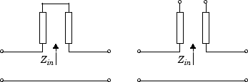
StubModeproperty to'Shunt', the 2-port network consists of a stub transmission line that you can terminate with either a short circuit or an open circuit as shown in the following figure.
Zin is the input impedance of the shunt circuit. The ABCD-parameters for the shunt stub are calculated as:
When you set the
StubModeproperty to'Series', the 2-port network consists of a series transmission line that you can terminate with either a short circuit or an open circuit as shown in the following figure.
Zin is the input impedance of the series circuit. The ABCD-parameters for the series stub are calculated as:
The analyze method uses the S-parameters to
calculate the group delay values at the frequencies specified in the
analyze input argument freq, as described in
the analyze reference page.
References
[1] Gupta, K. C., R. Garg, I. Bahl, and P. Bhartia, Microstrip Lines and Slotlines, 2nd Edition, Artech House, Inc., Norwood, MA, 1996.
Version History
Introduced before R2006a
See Also
rfckt.amplifier | rfckt.cascade | rfckt.coaxial | rfckt.datafile | rfckt.delay | rfckt.hybrid | rfckt.hybridg | rfckt.mixer | rfckt.microstrip | rfckt.passive | rfckt.parallel | rfckt.parallelplate | rfckt.rlcgline | rfckt.series | rfckt.seriesrlc | rfckt.shuntrlc | rfckt.twowire | rfckt.txline
