rfckt.twowire
Two-wire transmission line
Description
Use the rfckt.twowire object to create two-wire
transmission lines that are characterized by line dimensions, stub type, and
termination.
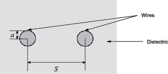
A two-wire transmission line is shown in cross-section in the following figure. Its physical characteristics include the radius of the wires a, the separation or physical distance between the wire centers S, and the relative permittivity and permeability of the wires. RF Toolbox™ software assumes the relative permittivity and permeability are uniform.
Note
txlineTwoWire is recommended over rfckt.twowire
because it enables you to:
Create a two-wire transmission line.
Build a
circuitobject with a two-wire transmission line.Model a two-wire transmission line element in an RF chain created using an
rfbudgetobject or the RF Budget Analyzer app, and then export this element to RF Blockset™ or torfsystemSystem object™ for circuit envelope analysis.
(since R2023b)
Creation
Description
h = rfckt.twowire returns a shunt RLC network object
whose properties all have their default values. The default object is
equivalent to a pass-through 2-port network; i.e., the resistor, inductor,
and capacitor are each replaced by a short circuit.
h = rfckt.twowire(Name,Value) sets properties using
one or more name-value pairs. For example,
rfckt.twowire('Radius',7.5e-4) creates a two-wire
transmission line with conducting wire radius of
7.5e-4 meters. You can specify multiple
name-value pairs. Enclose each property name in a quote. Properties not
specified retain their default values.
Properties
Object Functions
analyze | Analyze RFCKT object in frequency domain |
calculate | Calculate specified parameters for rfckt objects or rfdata objects |
circle | Draw circles on Smith Chart |
extract | Extract specified network parameters from rfckt object or data object |
listformat | List valid formats for specified circuit object parameter |
listparam | List valid parameters for specified circuit object |
loglog | Plot specified circuit object parameters using log-log scale |
plot | Plot circuit object parameters on X-Y plane |
plotyy | Plot parameters of RF circuit or RF data on xy-plane with two Y-axes |
getop | Display operating conditions |
polar | Plot specified object parameters on polar coordinates |
semilogx | Plot RF circuit object parameters using log scale for x-axis |
semilogy | Plot RF circuit object parameters using log scale for y-axis |
smith | Plot circuit object parameters on Smith Chart |
write | Write RF data from circuit or data object to file |
getz0 | Calculate characteristic impedance of RFCKT transmission line object |
read | Read RF data from file to new or existing circuit or data object |
restore | Restore data to original frequencies |
getop | Display operating conditions |
groupdelay | Group delay of S-parameter object or RF filter object or RF Toolbox circuit object |
Examples
Algorithms
If you model the transmission line as a stubless line, the
analyzemethod first calculates the ABCD-parameters at each frequency contained in the modeling frequencies vector. It then uses theabcd2sfunction to convert the ABCD-parameters to S-parameters.The
analyzemethod calculates the ABCD-parameters using the physical length of the transmission line, d, and the complex propagation constant, k, using the following equations:Z0 and k are vectors whose elements correspond to the elements of f, the vector of frequencies specified in the
analyzeinput argumentfreq. Both can be expressed in terms of the resistance (R), inductance (L), conductance (G), and capacitance (C) per unit length (meters) as follows:where
In these equations:
w is the plate width.
d is the plate separation.
σcond is the conductivity in the conductor.
μ is the permeability of the dielectric.
ε is the permittivity of the dielectric.
ε″ is the imaginary part of ε, ε″ = ε0εrtan δ, where:
ε0 is the permittivity of free space.
εr is the
EpsilonRproperty value.tan δ is the
LossTangentproperty value.
δcond is the skin depth of the conductor, which the block calculates as .
f is a vector of modeling frequencies determined by the Outport (RF Blockset) block.
If you model the transmission line as a shunt or series stub, the
analyzemethod first calculates the ABCD-parameters at the specified frequencies. It then uses theabcd2sfunction to convert the ABCD-parameters to S-parameters.When you set the
StubModeproperty to'Shunt', the 2-port network consists of a stub transmission line that you can terminate with either a short circuit or an open circuit as shown in the following figure.
Zin is the input impedance of the shunt circuit. The ABCD-parameters for the shunt stub are calculated as:
When you set the
StubModeproperty to'Series', the 2-port network consists of a series transmission line that you can terminate with either a short circuit or an open circuit as shown in the following figure.
Zin is the input impedance of the series circuit. The ABCD-parameters for the series stub are calculated as:
References
[1] Pozar, David M. Microwave Engineering, John Wiley & Sons, Inc., 2005.
Version History
Introduced in R2009a