Main Content

factorGraph

Bipartite graph of factors and nodes

Since R2022a

Description

A factorGraph object stores a bipartite graph consisting of factors connected to variable nodes. The nodes represent the unknown random variables in an estimation problem, such as robot poses, and the factors represent probabilistic constraints on those nodes, derived from measurements or prior knowledge. During optimization, the factor graph uses all the factors and current node states to update the node states.

To use the factor graph:

  1. Create an empty factorGraph object.

  2. For each desired factor type:

    1. Generate node IDs using the generateNodeID object function.

    2. Define factors with the desired node IDs, using any of the supported factor objects:

    3. Add factors to the factor graph using the addFactor object function. If the factor graph does not contain a node with the specified ID, the function automatically creates a node with that ID and adds it to the factor graph when adding the factor to the factor graph. If the factor graph contains a node with the specified ID, ensure that adding the new factor does not cause a node type mismatch. For more information, see Tips. For a list of expected node types for each factor, see Expected Node Types of Factor Objects.

  3. Check if all the nodes in the factor graph are connected to at least one other node using the isConnected object function.

  4. Create a factorGraphSolverOptions object to specify factor graph solver options.

  5. Optimize the factor graph using the optimize object function with the desired factor graph solver options.

  6. Extract factor graph node data, such as node IDs and node states, using the nodeIDs and nodeState object functions.

Creation

Description

example

fg = factorGraph creates an empty factorGraph object.

Properties

expand all

This property is read-only.

Number of nodes in the factor graph, specified as a positive integer. NumNodes has a value of 0 when the factor graph is empty and NumNodes increases each time you add a factor that specifies new node IDs to the factor graph.

The nodes in the factor graph can be any of these types:

  • "POSE_SE2" — Pose in SE(2) state space

  • "POSE_SE3" — Pose in SE(3) state space

  • "VEL3" — 3-D velocity

  • "POINT_XY" — 2-D point

  • "POINT_XYZ" — 3-D point

  • "IMU_BIAS" — IMU gyroscope and accelerometer bias

To check the node type of a node in the graph, use the nodeType function.

Note

The factor graph sets the node type when you add the factor object that specifies that node to the factor graph. You cannot change the node type of a node after you add it to the graph.

This property is read-only.

Number of factors in the factor graph, specified as a positive integer. NumFactors has a value of 0 when the factor graph is empty and NumFactors increases each time you add a factor to the factor graph.

You can use addfactor to add any of these factor objects to the factor graph:

Relate Poses to Sensor Measurements

  • factorGPS — Connect SE(3) pose node ("POSE_SE3") to a GPS measurement.

  • factorIMU — Connect two SE(3) pose nodes ("POSE_SE3"), two 3-D velocity nodes ("VEL3"), and two IMU bias nodes ("IMU_BIAS") using an IMU measurement.

Relate Poses to Landmark Positions

  • factorCameraSE3AndPointXYZ — Connect the SE(3) pose node of a pinhole camera ("POSE_SE3") to 3-D landmark nodes ("Point_XYZ") using relative pose measurements.

  • factorPoseSE2AndPointXY — Connect a SE(2) pose node ("POSE_SE2") to 2-D landmark nodes ("Point_XY") using relative pose measurements.

  • factorPoseSE3AndPointXYZ — Connect a SE(3) pose node ("POSE_SE3") to 3-D landmark nodes ("Point_XYZ") using relative pose measurements.

Relate Poses to Each Other

  • factorTwoPoseSE2 — Connect pairs of SE(2) pose nodes ("POSE_SE2") with relative poses using relative pose measurements.

  • factorTwoPoseSE3 — Connect pairs of SE(3) pose nodes ("POSE_SE3") with relative poses using relative pose measurements.

Relate Poses or Velocities to Prior-Known Measurements

  • factorIMUBiasPrior — Connect SE(3) pose nodes ("POSE_SE3"), 3-D velocity nodes ("VEL3"), and IMU bias nodes ("IMU_BIAS") to prior-known IMU measurements.

  • factorPoseSE3Prior — Connect SE(3) pose nodes ("POSE_SE3") to prior-known SE(3) pose measurements.

  • factorVelocity3Prior — Connect 3-D velocity node ("VEL_3") to prior-known SE(3) velocity measurements.

Object Functions

addFactorAdd factor to factor graph
fixNodeFix or free nodes in factor graph
generateNodeIDGenerate new node IDs
hasNodeCheck if node ID exists in factor graph
isConnectedCheck if factor graph is connected
isNodeFixedCheck if node is fixed
nodeIDsGet node IDs in factor graph
nodeStateGet or set node state in factor graph
nodeTypeGet node type of node in factor graph
optimizeOptimize factor graph
removeFactorRemove factor from factor graph
removeNodeRemove node from factor graph
showPlot pose nodes, pose node edges, and landmark nodes of factor graph

Examples

collapse all

Create a matrix of positions of the landmarks to use for localization, and the real poses of the robot to compare your factor graph estimate against. Use the exampleHelperPlotGroundTruth helper function to visualize the landmark points and the real path of the robot.

gndtruth = [0 0 0; 
            2 0 pi/2; 
            2 2 pi; 
            0 2 pi];
landmarks = [3 0; 0 3];
exampleHelperPlotGroundTruth(gndtruth,landmarks)

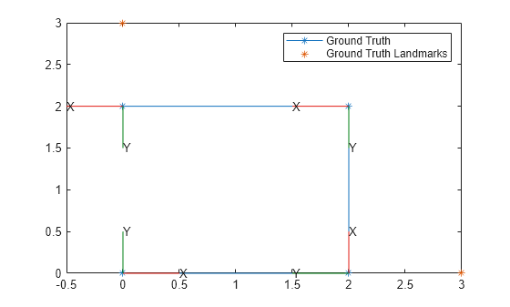
Use the exampleHelperSimpleFourPoseGraph helper function to create a factor graph contains four poses related by three 2-D two-pose factors. For more details, see the factorTwoPoseSE2 object page.

fg = exampleHelperSimpleFourPoseGraph(gndtruth);

Create Landmark Factors

Generate node IDs to create two node IDs for two landmarks. The second and third pose nodes observe the first landmark point so they should connect to that landmark with a factor. The third and fourth pose nodes observe the second landmark.

lmIDs = generateNodeID(fg,2);
lmFIDs = [1 lmIDs(1);  % Pose Node 1 <-> Landmark 1 
          2 lmIDs(1);  % Pose Node 2 <-> Landmark 1
          2 lmIDs(2);  % Pose Node 2 <-> Landmark 2
          3 lmIDs(2)]; % Pose Node 3 <-> Landmark 2

Define the relative position measurements between the position of the poses and their landmarks in the reference frame of the pose node. Then add some noise.

lmFMeasure = [0  -1; % Landmark 1 in pose node 1 reference frame 
             -1   2; % Landmark 1 in pose node 2 reference frame
              2  -1; % Landmark 2 in pose node 2 reference frame
              0  -1]; % Landmark 2 in pose node 3 reference frame
lmFMeasure = lmFMeasure + 0.1*rand(4,2);

Create the landmark factors with those relative measurements and add it to the factor graph.

lmFactor = factorPoseSE2AndPointXY(lmFIDs,Measurement=lmFMeasure);
addFactor(fg,lmFactor);

Set the initial state of the landmark nodes to the real position of the landmarks with some noise.

nodeState(fg,lmIDs,landmarks+0.1*rand(2));

Optimize Factor Graph

Optimize the factor graph with the default solver options. The optimization updates the states of all nodes in the factor graph, so the positions of vehicle and the landmarks update.

rng default
optimize(fg)
ans = struct with fields:
             InitialCost: 0.0538
               FinalCost: 6.2053e-04
      NumSuccessfulSteps: 4
    NumUnsuccessfulSteps: 0
               TotalTime: 1.6499e-04
         TerminationType: 0
        IsSolutionUsable: 1
        OptimizedNodeIDs: [1 2 3 4 5]
            FixedNodeIDs: 0

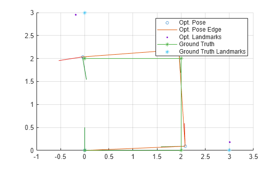
Visualize and Compare Results

Get and store the updated node states for the robot and landmarks. Then plot the results, comparing the factor graph estimate of the robot path to the known ground truth of the robot.

poseIDs = nodeIDs(fg,NodeType="POSE_SE2")
poseIDs = 1×4

     0     1     2     3

poseStatesOpt = nodeState(fg,poseIDs)
poseStatesOpt = 4×3

         0         0         0
    2.0815    0.0913    1.5986
    1.9509    2.1910   -3.0651
   -0.0457    2.0354   -2.9792

landmarkStatesOpt = nodeState(fg,lmIDs)
landmarkStatesOpt = 2×2

    3.0031    0.1844
   -0.1893    2.9547

handle = show(fg,Orientation="on",OrientationFrameSize=0.5,Legend="on");
grid on;
hold on;
exampleHelperPlotGroundTruth(gndtruth,landmarks,handle);

More About

expand all

Tips

  • To specify multiple factors and nodes at once for a specific factor type, use the generateNodeID function and specify the number of factors and the factor type. See the generateNodeID function for more details.

    poseIDPairs = generateNodeID(fg,3,"factorTwoPoseSE2");
    ftpse2 = factorTwoPoseSE2(poseIDPairs);
  • You can get the states of all the pose nodes by first using the nodeIDs function and specifying the node type as "POSE_SE2" for SE(2) robot poses and "POSE_SE3" for SE(3) robot poses. Then, use the nodeState function with those node IDs to get the node states of the robot pose nodes.

    poseIDs = nodeIDs(fg,NodeType="POSE_SE2");
    poseStates = nodeState(fg,poseIDs);
  • Check the types of nodes that each factor creates or connects to before adding factors to the factor graph to avoid node type mismatch errors. For a list of expected node types for each factor, see Expected Node Types of Factor Objects.

References

[1] Dellaert, Frank. Factor graphs and GTSAM: A Hands-On Introduction. Georgia: Georgia Tech, September, 2012.

Extended Capabilities

C/C++ Code Generation
Generate C and C++ code using MATLAB® Coder™.

Version History

Introduced in R2022a