pcolor

Pseudocolor plot

• 

Syntax

pcolor(C)

pcolor(X,Y,C)

pcolor(___,Name=Value)

pcolor(ax,___)

s = pcolor(___)

Description

pcolor(C) creates a pseudocolor plot using the values in matrix C. A pseudocolor plot displays matrix data as an array of colored cells (known as faces). MATLAB^® creates this plot as a flat surface in the x-y plane. The surface is defined by a grid of x- and y-coordinates that correspond to the corners (or vertices) of the faces. The grid covers the region X=1:n and Y=1:m, where [m,n] = size(C). Matrix C specifies the colors at the vertices. The color of each face depends on the color at one of its four surrounding vertices. Of the four vertices, the one that comes first in the x-y grid determines the color of the face.

pcolor(X,Y,C) specifies the x- and y-coordinates for the vertices. The size of C must match the size of the x-y coordinate grid. For example, if X and Y define an m-by-n grid, then C must be an m-by-n matrix.

pcolor(___,Name=Value) sets properties of the plot using one or more name-value arguments. For example, you can specify the color or hide the mesh lines of the plot. For a list of properties, see Surface Properties. (since R2024b)

pcolor(ax,___) specifies the target axes for the plot. Specify ax as the first argument in any of the previous syntaxes.

s = pcolor(___) returns a Surface object. Use s to set properties on the plot after creating it. For a list of properties, see Surface Properties.

Examples

Plot Four Faces with Four Colors

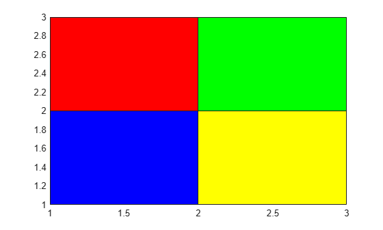
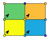
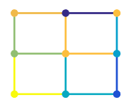
Create coordinate vectors X and Y and a colormap called mymap containing five colors: red, green, blue, yellow, and black.

X = [1 2 3; 1 2 3; 1 2 3];
Y = X';
mymap = [1 0 0; 0 1 0; 0 0 1; 1 1 0; 0 0 0];

Create matrix C that maps the colormap colors to the nine vertices. Four of the nine vertices determine the colors of the faces. Specify the colors at those vertices to make the faces red (1), green (2), blue (3), and yellow (4), respectively. Set the colors at the other vertices to black (5).

C = [3 4 5; 1 2 5; 5 5 5];

Plot the faces, and call the colormap function to replace the default colormap with mymap.

pcolor(X,Y,C)
colormap(mymap)

Plot Hadamard Matrix

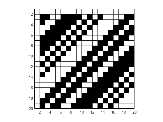
A Hadamard matrix has elements that are either 1 or -1. A good way to visualize this matrix is with a two-color colormap.

Create a 20-by-20 Hadamard matrix. Then plot the matrix using a black and white colormap. Use the axis function to reverse the direction of the y-axis and set the axis lines to equal lengths.

C = hadamard(20);
pcolor(C)
colormap(gray(2))
axis ij
axis square

Modify Borders

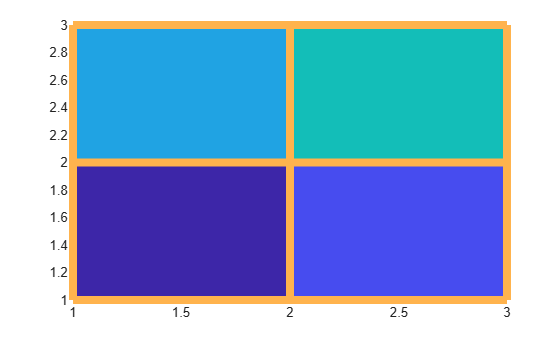
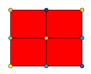
Create color matrix C. Then create a pseudocolor plot of C, and store the Surface object in the return argument s.

C = [1 2 3; 4 5 6; 7 8 9];
s = pcolor(C);

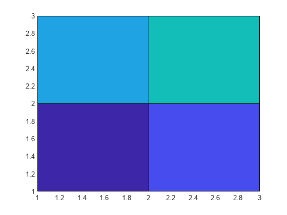
Change the border color by setting the EdgeColor property of s. Make the border thicker by setting the LineWidth property.

s.EdgeColor = [1 0.7 0.3];
s.LineWidth = 6;

Interpolate Colors Across Faces

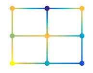
Create color matrix C. Then create a pseudocolor plot of C, and store the Surface object in the return argument s.

C = [5 13 9 7 12; 11 2 14 8 10; 6 1 3 4 15];
s = pcolor(C);

To interpolate the colors across the faces, set the FaceColor property of s to 'interp'.

s.FaceColor = 'interp';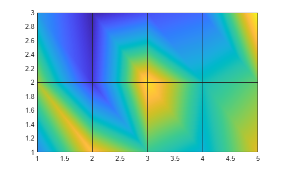

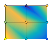
Specify Semilogarithmic Grid

Create matrices X and Y, which define a regularly spaced grid of vertices. Calculate matrix LY as the log of Y. Then create matrix C containing alternating pairs of rows of color indices.

[X,Y] = meshgrid(1:20);
LY = log(Y);
colorscale = [1:20; 20:-1:1];
C = repmat(colorscale,10,1);

Plot X and LY, using the colors specified in C. Then adjust the tick labels on the y-axis.

s = pcolor(X,LY,C);
tickvals = LY(2:2:20,1)';
set(gca,'YTick',tickvals);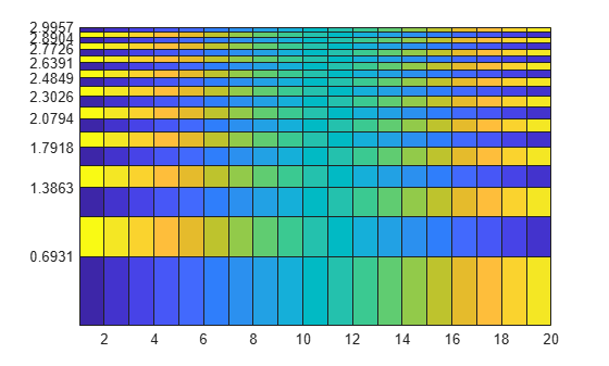

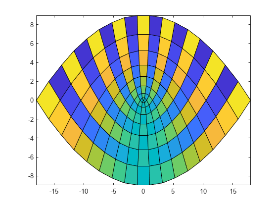
Specify Parametric Grid

Create matrices X and Y, which define a regularly spaced grid of vertices. Calculate matrices XX and YY as functions of X and Y. Then create matrix C containing alternating pairs of rows of color indices.

[X,Y] = meshgrid(-3:6/17:3);
XX = 2*X.*Y;
YY = X.^2 - Y.^2;
colorscale = [1:18; 18:-1:1];
C = repmat(colorscale,9,1);

Plot XX and YY using the colors in C.

pcolor(XX,YY,C);

Specify Target Axes

Call the tiledlayout function to create a 1-by-2 tiled chart layout. Call the nexttile function to create the axes objects ax1 and ax2. Create two pseudocolor plots by specifying the axes as the first argument to pcolor.

tiledlayout(1,2)

% Left plot
ax1 = nexttile;
C1 = rand(20,10);
pcolor(ax1,C1)

% Right plot
ax2 = nexttile;
C2 = rand(50,10);
pcolor(ax2,C2)

Input Arguments

C — Color matrix

matrix

Color matrix containing indices into the colormap. The values in C map colors in the colormap array to the vertices surrounding each face. The color of a face depends on the color at one of its four vertices. Of the four vertices, the one that come first in X and Y determines the color of the face. If you do not specify X and Y, MATLAB uses X=1:n and Y=1:m, where [m,n] = size(C). Because of this relationship between the vertex colors and face colors, none of the values in the last row and column of C are represented in the plot.

Note

The first vertex of a face is the one that is closest to the upper-left corner of the corresponding matrix. However, because the y-axis increases from bottom to top, the first vertex shown in the plot is typically the one in the lower-left corner of the face. To get the effect you want, you might have to change the orientation of the y-axis or the orientation of matrix C.

For a simple example that shows the relationship between the colors of the vertices and the faces, see Plot Four Faces with Four Colors.

The values in C scale to the full range of the colormap. The smallest value in C maps to the first row in the colormap array. The largest value in C maps to the last row in the colormap array. The intermediate values in C map linearly to the intermediate rows of the colormap array. You can adjust this mapping using the clim function.

Before R2022a: Use the caxis function, which has the same syntaxes and arguments as clim.

The CData property of the Surface object stores the values of C.

Data Types: single | double | int8 | int16 | int32 | int64 | uint8 | uint16 | uint32 | uint64

X — x-coordinates

matrix | vector

x-coordinates, specified as a matrix the same size as C, or as a vector of length n, where [m,n] = size(C). The default value of X is the vector (1:n).

To create a rectangular grid of vertices, specify X as either of the following:

• A vector containing values that are increasing or decreasing.

• A matrix that is increasing or decreasing along one dimension and is constant along the other dimension. Set the dimension that varies to the opposite of the dimension that varies in matrix Y. You can use the meshgrid function to create the X and Y matrices.

To create a parametric grid, create a rectangular grid and pass it through a mathematical function.

Example: X = 1:10

Example: X = [1 2 3; 1 2 3; 1 2 3]

Example: [X,Y] = meshgrid(1:10)

The XData property of the Surface object stores the x-coordinates.

Data Types: single | double | int8 | int16 | int32 | int64 | uint8 | uint16 | uint32 | uint64 | categorical | datetime | duration

Y — y-coordinates

matrix | vector

y-coordinates, specified as a matrix the same size as C, or as a vector of length m, where [m,n] = size(C). The default value of Y is the vector (1:m).

To create a rectangular grid of vertices, specify Y as either of the following:

• A vector containing values that are increasing or decreasing.

• A matrix that is increasing or decreasing along one dimension and is constant along the other dimension. Set the dimension that varies to the opposite of the dimension that varies in matrix X. You can use the meshgrid function to create the X and Y matrices.

To create a parametric grid, create a rectangular grid and pass it through a mathematical function.

Example: Y = 1:10

Example: Y = [1 1 1; 2 2 2; 3 3 3]

Example: [X,Y] = meshgrid(1:10)

The YData property of the Surface object stores the y-coordinates.

Data Types: single | double | int8 | int16 | int32 | int64 | uint8 | uint16 | uint32 | uint64 | categorical | datetime | duration

ax — Target axes

Axes object

Target axes, specified as an Axes object. If you do not specify the axes, then pcolor plots into the current axes.

Name-Value Arguments

Specify optional pairs of arguments as Name1=Value1,...,NameN=ValueN, where Name is the argument name and Value is the corresponding value. Name-value arguments must appear after other arguments, but the order of the pairs does not matter.

Example: pcolor([1 2 3; 4 5 6; 7 8 9],FaceColor="interp") interpolates the color across the faces.

Note

The properties listed here are only a subset. For a full list, see Surface Properties.

FaceColor — Face color

'flat' (default) | 'interp' | 'none' | 'texturemap' | RGB triplet | hexadecimal color code | 'r' | 'g' | 'b' | ...

Face color, specified as one of the values in this table.

Value	Description
'flat'	Use a different color for each face based on the values in the CData property. First you must specify the CData property as a matrix the same size as ZData. The color value at the first vertex of each face (in the positive x and y directions) determines the color for the entire face. You cannot use this value when the FaceAlpha property is set to 'interp'.
'interp'	Use interpolated coloring for each face based on the values in the CData property. First you must specify the CData property as a matrix the same size as ZData. The color varies across each face by interpolating the color values at the vertices. You cannot use this value when the FaceAlpha property is set to 'flat'.
RGB triplet, hexadecimal color code, or color name	Use the specified color for all the faces. This option does not use the color values in the CData property.
'texturemap'	Transform the color data in CData so that it conforms to the surface.
'none'	Do not draw the faces.

RGB triplets and hexadecimal color codes are useful for specifying custom colors.

• An RGB triplet is a three-element row vector whose elements specify the intensities of the red, green, and blue components of the color. The intensities must be in the range [0,1]; for example, [0.4 0.6 0.7].

• A hexadecimal color code is a character vector or a string scalar that starts with a hash symbol (#) followed by three or six hexadecimal digits, which can range from 0 to F. The values are not case sensitive. Thus, the color codes "#FF8800", "#ff8800", "#F80", and "#f80" are equivalent.

Alternatively, you can specify some common colors by name. This table lists the named color options, the equivalent RGB triplets, and hexadecimal color codes.

Color Name	Short Name	RGB Triplet	Hexadecimal Color Code	Appearance
"red"	"r"	[1 0 0]	"#FF0000"
"green"	"g"	[0 1 0]	"#00FF00"
"blue"	"b"	[0 0 1]	"#0000FF"
"cyan"	"c"	[0 1 1]	"#00FFFF"
"magenta"	"m"	[1 0 1]	"#FF00FF"
"yellow"	"y"	[1 1 0]	"#FFFF00"
"black"	"k"	[0 0 0]	"#000000"
"white"	"w"	[1 1 1]	"#FFFFFF"

Here are the RGB triplets and hexadecimal color codes for the default colors MATLAB uses in many types of plots.

RGB Triplet	Hexadecimal Color Code	Appearance
[0 0.4470 0.7410]	"#0072BD"
[0.8500 0.3250 0.0980]	"#D95319"
[0.9290 0.6940 0.1250]	"#EDB120"
[0.4940 0.1840 0.5560]	"#7E2F8E"
[0.4660 0.6740 0.1880]	"#77AC30"
[0.3010 0.7450 0.9330]	"#4DBEEE"
[0.6350 0.0780 0.1840]	"#A2142F"

EdgeColor — Edge line color

[0 0 0] (default) | 'none' | 'flat' | 'interp' | RGB triplet | hexadecimal color code | 'r' | 'g' | 'b' | ...

Edge line color, specified as one of the values listed here. The default color of [0 0 0] corresponds to black edges.

Value	Description
'none'	Do not draw the edges.
'flat'	Use a different color for each edge based on the values in the CData property. First you must specify the CData property as a matrix the same size as ZData. The color value at the first vertex of each face (in the positive x and y directions) determines the color for the adjacent edges. You cannot use this value when the EdgeAlpha property is set to 'interp'.
'interp'	Use interpolated coloring for each edge based on the values in the CData property. First you must specify the CData property as a matrix the same size as ZData. The color varies across each edge by linearly interpolating the color values at the vertices. You cannot use this value when the EdgeAlpha property is set to 'flat'.
RGB triplet, hexadecimal color code, or color name	Use the specified color for all the edges. This option does not use the color values in the CData property.

RGB triplets and hexadecimal color codes are useful for specifying custom colors.

• An RGB triplet is a three-element row vector whose elements specify the intensities of the red, green, and blue components of the color. The intensities must be in the range [0,1]; for example, [0.4 0.6 0.7].

• A hexadecimal color code is a character vector or a string scalar that starts with a hash symbol (#) followed by three or six hexadecimal digits, which can range from 0 to F. The values are not case sensitive. Thus, the color codes "#FF8800", "#ff8800", "#F80", and "#f80" are equivalent.

Alternatively, you can specify some common colors by name. This table lists the named color options, the equivalent RGB triplets, and hexadecimal color codes.

Color Name	Short Name	RGB Triplet	Hexadecimal Color Code	Appearance
"red"	"r"	[1 0 0]	"#FF0000"
"green"	"g"	[0 1 0]	"#00FF00"
"blue"	"b"	[0 0 1]	"#0000FF"
"cyan"	"c"	[0 1 1]	"#00FFFF"
"magenta"	"m"	[1 0 1]	"#FF00FF"
"yellow"	"y"	[1 1 0]	"#FFFF00"
"black"	"k"	[0 0 0]	"#000000"
"white"	"w"	[1 1 1]	"#FFFFFF"

Here are the RGB triplets and hexadecimal color codes for the default colors MATLAB uses in many types of plots.

RGB Triplet	Hexadecimal Color Code	Appearance
[0 0.4470 0.7410]	"#0072BD"
[0.8500 0.3250 0.0980]	"#D95319"
[0.9290 0.6940 0.1250]	"#EDB120"
[0.4940 0.1840 0.5560]	"#7E2F8E"
[0.4660 0.6740 0.1880]	"#77AC30"
[0.3010 0.7450 0.9330]	"#4DBEEE"
[0.6350 0.0780 0.1840]	"#A2142F"

LineStyle — Line style

"-" (default) | "--" | ":" | "-." | "none"

Line style, specified as one of the options listed in this table.

Line Style	Description	Resulting Line
"-"	Solid line
"--"	Dashed line
":"	Dotted line
"-."	Dash-dotted line
"none"	No line	No line

Algorithms

Use the pcolor, image, and imagesc functions to display rectangular arrays of colored cells. The relationship between the color matrix C and the colored cells is different in each case.

• pcolor(C) uses the values in C to define the vertex colors by scaling the values to the full range of the colormap. The size of C determines the number of vertices. The values in C map colors from the current colormap to the vertices surrounding each cell.

• image(C) uses C to define the cell colors by mapping the values directly into the colormap. The size of C determines the number of cells.

• imagesc(C) uses C to define the cell colors by scaling the values to the full range of the colormap. The size of C determines the number of cells.

Extended Capabilities

GPU Arrays

Accelerate code by running on a graphics processing unit (GPU) using Parallel Computing Toolbox™.

The pcolor function supports GPU array input with these usage notes and limitations:

• This function accepts GPU arrays, but does not run on a GPU.

For more information, see Run MATLAB Functions on a GPU (Parallel Computing Toolbox).

Distributed Arrays

Partition large arrays across the combined memory of your cluster using Parallel Computing Toolbox™.

Usage notes and limitations:

• This function operates on distributed arrays, but executes in the client MATLAB.

For more information, see Run MATLAB Functions with Distributed Arrays (Parallel Computing Toolbox).

Version History

Introduced before R2006a

R2024b: Control appearance and behavior with name-value arguments

Control the appearance and behavior of pseudocolor plots by specifying name-value arguments. Previously, pcolor did not support name-value arguments.