pem
Prediction error minimization for refining linear and nonlinear models
Description
sys = pem(data,init_sys)init_sys to fit the estimation
data in data. data can be a timetable, a
comma-separated pair of matrices, or a data object.
The function uses prediction-error minimization algorithm to update the parameters of the initial model. Use this command to refine the parameters of a previously estimated model.
Examples
Estimate a discrete-time state-space model using n4sid, which applies the subspace method.
Load the data and extract the first 300 points for the estimation data.
load sdata7 tt7;
tt7e = tt7(1:300,:);
Estimate the model init_sys, setting the 'Focus' option to 'simulation'.
opt = n4sidOptions('Focus','simulation');
init_sys = n4sid(tt7e,4,opt);
Show the estimation fit.
init_sys.Report.Fit.FitPercent
ans =
73.8490
Use pem to improve the closeness of the fit.
sys = pem(tt7e,init_sys);
Analyze the results.
compare(tt7e,sys,init_sys);
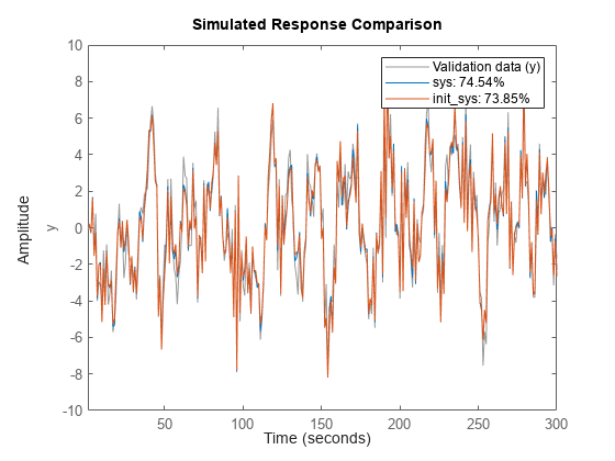
Using pem improves the fit to the estimation data.
Estimate the parameters of a nonlinear grey-box model to fit DC motor data.
Load the experimental data, and specify the signal attributes such as start time and units.
load('dcmotordata');
data = iddata(y, u, 0.1);
data.Tstart = 0;
data.TimeUnit = 's';
Configure the nonlinear grey-box model (idnlgrey) model.
For this example, use dcmotor_m.m file. To view this file, type edit dcmotor_m.m at the MATLAB® command prompt.
file_name = 'dcmotor_m';
order = [2 1 2];
parameters = [1;0.28];
initial_states = [0;0];
Ts = 0;
init_sys = idnlgrey(file_name,order,parameters,initial_states,Ts);
init_sys.TimeUnit = 's';

setinit(init_sys,'Fixed',{false false});
init_sys is a nonlinear grey-box model with its structure described by dcmotor_m.m. The model has one input, two outputs and two states, as specified by order.
setinit(init_sys,'Fixed',{false false}) specifies that the initial states of init_sys are free estimation parameters.
Estimate the model parameters and initial states.
sys = pem(data,init_sys);
sys is an idnlgrey model, which encapsulates the estimated parameters and their covariance.
Analyze the estimation result.
compare(data,sys,init_sys);
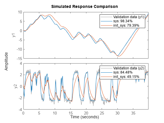
sys provides a 98.34% fit to the estimation data.
Create a process model structure and update its parameter values to minimize prediction error.
Initialize the coefficients of a process model.
init_sys = idproc('P2UDZ');
init_sys.Kp = 10;
init_sys.Tw = 0.4;
init_sys.Zeta = 0.5;
init_sys.Td = 0.25;
init_sys.Tz = 0.01;
The Kp, Tw, Zeta, Td, and Tz coefficients of init_sys are configured with their initial guesses.
Use init_sys to configure the estimation of a prediction error minimizing model using measured data. Because init_sys is an idproc model, use procestOptions to create the option set.
load iddata1 z1;
opt = procestOptions('Display','on','SearchMethod','lm');
sys = pem(z1,init_sys,opt);
Process Model Identification

Estimation data: Time domain data z1
Data has 1 outputs, 1 inputs and 300 samples.
Model Type:
    {'P2DUZ'}


Algorithm: Levenberg-Marquardt search
 <br>
------------------------------------------------------------------------------------------
 <br>
                          Norm of      First-order    Improvement (%) <br> Iteration       Cost       step         optimality     Expected   Achieved    Bisections <br>------------------------------------------------------------------------------------------
     0        29.7194          -            260        2.57           -         -
     1        28.6801          6           98.9        2.57         3.5         0
     2        8.38196       4.91           42.2        2.72        70.8         0
     3         8.2138      0.704           41.3        1.37        2.01        12
     4        8.00237      0.528           48.3        2.89        2.57         9
     5        7.65577      0.588           73.1        2.02        4.33         9
     6          6.851      0.809            196        4.51        10.5         9
     7        5.72335       1.08            459        4.59        16.5         8
     8         3.3434       2.11       1.63e+03        11.4        41.6         7
     9        1.80724      0.701            504        14.2        45.9         0
    10         1.6812      0.122             12        4.24        6.97         0
    11        1.68092      0.014           1.11       0.309      0.0168         0
    12        1.68092    0.00179         0.0215         0.3    0.000101         0
    13        1.68092   0.000112        0.00634         0.3    8.26e-07         0
    14        1.68092   1.36e-05       0.000382         0.3    7.62e-09         0
    15        1.68092   1.18e-06       5.01e-05         0.3    7.28e-11         0
    16        1.68092   1.23e-07       4.29e-06         0.3    7.13e-13         0
    17        1.68092   1.17e-08       4.56e-07         0.3    1.32e-14         0
------------------------------------------------------------------------------------------
Termination condition: No improvement along the search direction with line search..
Number of iterations: 18, Number of function evaluations: 115

Status: Estimated using PEM
Fit to estimation data: 70.57%, FPE: 1.7379
Examine the model fit.
sys.Report.Fit.FitPercent
ans =
       70.567
sys provides a 70.63% fit to the measured data.
Input Arguments
Output Arguments
Algorithms
PEM uses numerical optimization to minimize the cost function, a weighted norm of the prediction error, defined as follows for scalar outputs:
where e(t) is the difference between the measured output and the predicted output of the model. For a linear model, the error is defined as:
where e(t) is a vector and the cost function is a scalar value. The subscript N indicates that the cost function is a function of the number of data samples and becomes more accurate for larger values of N. For multiple-output models, the previous equation is more complex. For more information, see chapter 7 in System Identification: Theory for the User, Second Edition, by Lennart Ljung, Prentice Hall PTR, 1999.
Alternative Functionality
You can achieve the same results as pem by using dedicated estimation
commands for the various model structures. For example, use ssest(data,init_sys) for estimating state-space models.
Version History
Introduced before R2006a