VAR Model Estimation Overview

Open Live Script

Decide on a set of VAR candidates to models, fit each model to the data, choose the model with the best fit, and then determine whether the AR polynomial of the estimated model is stable. Econometrics Toolbox™ has several functions that aid these tasks, including:

estimate — Fit VAR model to data.
summarize — Display and returns parameter estimates and other summary statistics from an estimated model.
lratiotest or aicbic — Determine the adequate number of lags by comparing the fit statistics of fitted models.
infer — Compute residuals of an estimated model for diagnostic checking.
forecast — Determine the predictive performance of a model by comparing forecasts to observed responses (see VAR Model Forecasting, Simulation, and Analysis)
LagOpand isStable — Determine whether an AR polynomial is stable.

Load Multivariate Economic Data

Load the US macroeconomic data. Consider modeling the joint dynamics of the US gross domestic product (GDP), consumer price index (CPI), and unemployment rate series, and suppose government consumption expenditures is an exogenous variable. For more details on the data, see Format Multivariate Time Series Data.

load Data_USEconModel
ynames = ["CPIAUCSL" "UNRATE" "GDP"];
xnames = "GCE";
DTT = DataTimeTable(:,[ynames xnames]);

Prepare Data for Estimation

To fit a VAR model to your data, you must format, preprocess, and partition the multivariate data for estimation (see Format Multivariate Time Series Data).

Format: varm object functions accept data in matrices, tables, or timetables. For timetables, row dates must be regular. Although the US macroeconomic data set contains the series in all those forms, the row dates of the timetable DataTimeTable do not comprise a regular series. Because this example uses the timetable, the example addresses the irregular dates.
Preprocess: When you plan to supply a timetable of data to varm functions, you must ensure that the selected response variables are numeric, do not contain any missing values, and the timestamps in the Time variable are regular and in ascending or descending order. Also, the series must be stationary.
Partition: This example creates a set of candidate VAR( $p$ ) models, where the order $p$ and lag terms present in the model vary. $p$ determines the required number of presample observations to initialize the model. This example uses a maximum of $p = 8$ ; therefore the presample is the first 8 observations for all models. This example uses the AIC to determine the best fitting model. Therefore, this example fits the models to the remaining observations. However, you can partition the data further to use out-of-sample forecast measures to compare the models' predictive performance. How you partition the data depends on your analysis goals.

Remove Missing Values

Remove the observations from the head of the table that contain consecutive missing values.

DTT = rmmissing(DTT);

rmmissing uses listwise deletion to remove all rows from the input timetable containing at least one missing observation.

Regularize Sample Dates

Determine whether the sampling timestamps have a regular frequency and are sorted.

areTimestampsRegular = isregular(DTT,"quarters")

areTimestampsRegular = logical
   0

areTimestampsSorted = issorted(DTT.Time)

areTimestampsSorted = logical
   1

areTimestampsRegular = 0 indicates that the timestamps of DTT are irregular. areTimestampsSorted = 1 indicates that the timestamps are sorted. Macroeconomic series in this example are timestamped at the end of the month. This quality induces an irregularly measured series.

Remedy the time irregularity by shifting all dates to the first day of the quarter.

dt = DTT.Time;
dt = dateshift(dt,"start","quarter");
DTT.Time = dt;
areTimestampsRegular = isregular(DTT,"quarters")

areTimestampsRegular = logical
   1

DTT is regular.

Stabilize the Series

Econometrics Toolbox has a variety of functions that conduct statistical tests for stationary (see Unit Root Nonstationarity). This example inspects plots of the time series to determine whether the series must be stabilized.

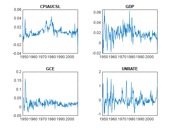
Plot the response and predictor series in separate plots.

tiledlayout(2,2)
for j = 1:width(DTT)
    nexttile
    plot(DTT.Time,DTT{:,j})
    title(DTT.Properties.VariableNames(j))
end

By visual inspection:

The CPI, GDP, and GCE series exponentially increase. This example converts these series to rates (percents) by using price2ret.
The unemployment rate series appears nonstationary. This example applies the first difference to the series.

Stabilize the series. Plot the stabilized series.

DTTt = price2ret(DTT,DataVariables=["CPIAUCSL" "GDP" "GCE"]);
DTTt.Variables = DTTt.Variables*100;
DTTt.UNRATE = diff(DTT.UNRATE);
DTTt.Interval = [];

tiledlayout(2,2)
for j = 1:width(DTT)
    nexttile
    plot(DTTt.Time,DTTt{:,j})
    title(DTTt.Properties.VariableNames(j))
end

Figure contains 4 axes objects. Axes object 1 with title CPIAUCSL contains an object of type line. Axes object 2 with title GDP contains an object of type line. Axes object 3 with title GCE contains an object of type line. Axes object 4 with title UNRATE contains an object of type line.

Application of the first difference and conversion to rates reducing the effective sample size by 1.

Partition the Data

A VAR model with maximum order of 8 model requires 8 presample responses. Partition the data into presample and estimation samples.

maxp = 8;           % Num. presample observations
T = height(DTTt);   % Total sample size
eT = T - maxp;      % Effective sample size

idxpre = 1:maxp;
idxest = (maxp + 1):T;

DTT0 = DTTt(idxpre,:);  % Presample
DTTE = DTTt(idxest,:);  % Estimation sample

Specify Candidate VARX Models

Specify the candidate VARX models in the table, containing estimable parameters, by calling the varm function (see Vector Autoregression (VAR) Model Creation). Each model contains an estimable constant and innovations covariance matrix.

	$Φ_{1}$	$Φ_{4}$	$Φ_{8}$
$VARX (0)$
${VARX (8)}_{1}$			x
${VARX (4)}_{1}$		x
${VARX (8)}_{2}$		x	x
$VARX (1)$	x
${VARX (8)}_{3}$	x		x
${VARX (4)}_{2}$	x	x
${VARX (8)}_{4}$	x	x	x

Create a design matrix that identifies which coefficients are present in the model.

numseries = numel(ynames);
CoeffIdx = logical(ff2n(numseries))

CoeffIdx = 8×3 logical array

   0   0   0
   0   0   1
   0   1   0
   0   1   1
   1   0   0
   1   0   1
   1   1   0
   1   1   1

nummdls = height(CoeffIdx);

Create the VARX models in a for loop. Store the models in a vector.

lags = [1 4 8];
Mdls(8) = varm(numseries,0); % Preallocate model vector
for j = 1:nummdls
    coeffidx = lags(CoeffIdx(j,:));
    Mdls(j) = varm(Constant=NaN(numseries,1),Lags=coeffidx, ...
        SeriesNames=ynames);
end
Mdls(4)

ans = 
  varm with properties:

     Description: "3-Dimensional VAR(8) Model"
     SeriesNames: "CPIAUCSL"  "UNRATE"  "GDP" 
       NumSeries: 3
               P: 8
        Constant: [3×1 vector of NaNs]
              AR: {3×3 matrices} at lags [4 8]
           Trend: [3×1 vector of zeros]
            Beta: [3×0 matrix]
      Covariance: [3×3 matrix of NaNs]

Mdls(4).AR'

ans=8×1 cell array
    {3×3 double}
    {3×3 double}
    {3×3 double}
    {3×3 double}
    {3×3 double}
    {3×3 double}
    {3×3 double}
    {3×3 double}

Mdls is an 8-by-1 vector of varm objects containing estimable parameters. Mdls(4) matches the structure of the fourth model in the table. Lags 4 and 8 of the model contain coefficient matrices of NaN values, which indicates that they are estimable. All other lags have coefficient matrices of zeros, which means that they are effectively absent from the model. The Beta property is an empty matrix; MATLAB® populates Beta during estimation when you specify predictor data.

Fit Models to Data

The estimate function fits an input varm model containing estimable parameters to input data.

Estimate all VARX models in the vector. Store the results in a vector of estimated varm objects. Obtain the AIC of each fit by extracting that statistic from the output of summarize. Specify the entire presample for each estimation.

for j = nummdls:-1:1
    EstMdls(j) = estimate(Mdls(j),DTTE,ResponseVariables=ynames, ...
        PredictorVariables=xnames,Presample=DTT0);
    StatsEstMdls(j) = summarize(EstMdls(j));
    ic(j) = StatsEstMdls(j).AIC;
end
EstMdls(4)

ans = 
  varm with properties:

     Description: "AR-Stationary 3-Dimensional VARX(8) Model with 1 Predictor"
     SeriesNames: "CPIAUCSL"  "UNRATE"  "GDP" 
       NumSeries: 3
               P: 8
        Constant: [0.0016423 -0.0396456 0.010304]'
              AR: {3×3 matrices} at lags [4 8]
           Trend: [3×1 vector of zeros]
            Beta: [3×1 matrix]
      Covariance: [3×3 matrix]

EstMdls is an 8-by-1 vector of varm objects; EstMdls(j) represents the estimated VAR model corresponding to the model structure Mdls(j). You can access parameter estimates by using dot notation. For example, display the exogenous regression coefficient matrix estimate and the lag 4 coefficient matrix.

EstMdls(4).SeriesNames

ans = 1×3 string
    "CPIAUCSL"    "UNRATE"    "GDP"

Beta = EstMdls(4).Beta

Beta = 3×1

    0.1184
   -3.6739
    0.2186

Phi4 = EstMdls(4).AR{4}

Phi4 = 3×3

    0.3060   -0.0012    0.0506
   12.4739   -0.2332    1.5961
   -0.0966    0.0058    0.0054

The rows and columns of the parameters correspond to the series in EstMdls(4).SeriesNames.

How `estimate` Works

Before fitting the model to data, estimate requires at least $p$ presample observations to initialize the model. varm stores the model degree $p$ in property P of the varm model object. This example specifies the presample so that the models can be fairly compared, but, by default, estimate removes the first P observations from the specified estimation sample. Therefore, if you let estimate take requisite presample observations from the input estimation sample data, the effective sample size decreases.

estimate computes maximum likelihood estimates of the parameters present in the model. Specifically, estimate fits the estimable parameters corresponding to the varm model properties Constant, AR, Trend, Beta, and Covariance. For VAR models, estimate uses a direct solution algorithm that requires no iterations. For VARX models, estimate optimizes the likelihood using the expectation-conditional-maximization (ECM) algorithm. The iterations usually converge quickly, unless two or more exogenous data streams are proportional to each other. In that case, no unique maximum likelihood estimator exists, and, consequently, the algorithm might not converge on a solution. You can set the maximum number of iterations with the MaxIterations name-value argument, which has a default value of 1000.

Unlike univariate conditional mean and variance model estimation (for example, arima and garch model estimation), estimate performs unrestricted maximum likelihood. Therefore, estimate can return an unstable VAR model.

For numeric array data inputs, estimate removes entire observations from the data containing at least one missing value (NaN). For table or timetable data inputs, estimate issues an error when any observation is missing. For more details, see estimate.

estimate calculates the loglikelihood of the data, and then returns it as an output of the fitted model. You can use this output in testing the quality of the model. For example, see Select Appropriate Lag Order.

Choose Best Fitting Model

Choose the model with the best fit by finding the estimated model that minimizes the AIC.

[~,bestIdx] = min(ic)

bestIdx = 
8

The best fitting model is the VARX(8) model that includes lags $Φ_{1}$ , $Φ_{4}$ , and $Φ_{8}$ .

Summarize the best fitting model.

BestFitEstMdl = EstMdls(bestIdx);
summarize(BestFitEstMdl)

 
   AR-Stationary 3-Dimensional VARX(8) Model with 1 Predictor
 
    Effective Sample Size: 236
    Number of Estimated Parameters: 33
    LogLikelihood: 1580.02
    AIC: -3094.04
    BIC: -2979.73
 
                      Value       StandardError    TStatistic      PValue  
                   ___________    _____________    __________    __________

    Constant(1)     0.00042224      0.0014111        0.29923        0.76477
    Constant(2)       0.083343       0.066472         1.2538        0.20991
    Constant(3)      0.0080822      0.0018504         4.3678      1.255e-05
    AR{1}(1,1)         0.38803       0.070814         5.4796     4.2641e-08
    AR{1}(2,1)          5.6013         3.3358         1.6791       0.093124
    AR{1}(3,1)         0.19235        0.09286         2.0714       0.038323
    AR{1}(1,2)     -0.00011792      0.0015733      -0.074949        0.94026
    AR{1}(2,2)         0.28432       0.074114         3.8362     0.00012494
    AR{1}(3,2)      -0.0070376      0.0020631        -3.4111     0.00064697
    AR{1}(1,3)         0.10432       0.059929         1.7407       0.081729
    AR{1}(2,3)          -8.662         2.8231        -3.0683      0.0021531
    AR{1}(3,3)         0.15497       0.078588         1.9719       0.048618
    AR{4}(1,1)         0.11635       0.075627         1.5384        0.12395
    AR{4}(2,1)           7.344         3.5626         2.0614       0.039261
    AR{4}(3,1)        -0.12058       0.099172        -1.2158        0.22405
    AR{4}(1,2)      -0.0012109      0.0015642       -0.77417        0.43883
    AR{4}(2,2)        -0.20262       0.073684        -2.7499      0.0059612
    AR{4}(3,2)       0.0052556      0.0020512         2.5623       0.010399
    AR{4}(1,3)         0.02242       0.059003        0.37998        0.70396
    AR{4}(2,3)         0.70129         2.7795        0.25231         0.8008
    AR{4}(3,3)      -0.0090903       0.077373       -0.11749        0.90647
    AR{8}(1,1)        0.071877       0.067845         1.0594         0.2894
    AR{8}(2,1)         0.37516          3.196        0.11738        0.90656
    AR{8}(3,1)         0.13963       0.088968         1.5695        0.11654
    AR{8}(1,2)      0.00015779      0.0015394         0.1025        0.91836
    AR{8}(2,2)        -0.19092       0.072518        -2.6326      0.0084722
    AR{8}(3,2)         0.00618      0.0020187         3.0614      0.0022032
    AR{8}(1,3)         0.02496       0.055678         0.4483        0.65394
    AR{8}(2,3)         -1.8024         2.6229       -0.68718        0.49197
    AR{8}(3,3)         0.13983       0.073013         1.9151       0.055475
    Beta(1,1)         0.058412       0.026055         2.2419       0.024966
    Beta(2,1)          -1.5393         1.2274        -1.2542        0.20978
    Beta(3,1)          0.14514       0.034166          4.248     2.1573e-05

 
   Innovations Covariance Matrix:
    0.0000   -0.0000    0.0000
   -0.0000    0.1107   -0.0017
    0.0000   -0.0017    0.0001

 
   Innovations Correlation Matrix:
    1.0000   -0.0123    0.2560
   -0.0123    1.0000   -0.5376
    0.2560   -0.5376    1.0000

Examine Stability of AR Polynomial

When you enter the name of a fitted model at the command line, you obtain an object summary. In the Description row of the summary (which shows the value of the Description property), varm indicates whether the VAR model (or, the AR polynomial of the model) is stable.

Another way to determine whether a VAR model is stationary of the VAR model is to create a lag operator polynomial object using the estimated autoregression coefficients (see LagOp), and then passing the lag operator to the isStable function.

Determine whether the best fitting model BestFitEstMdl is stable using lag operator polynomial objects. Observe that LagOp requires the coefficient of lag 0.

AR = [{eye(numseries)} BestFitEstMdl.AR];   % Include the lag 0 coefficient.
Mdl = LagOp(AR);
Mdl = reflect(Mdl);                         % Negate all lags > 0
isStable(Mdl)

ans = logical
   1

isStable returns the logical value 1, indicating that the best fitting model is stable. Regression components can destabilize an otherwise stable VAR model. This process determines the stability of the VAR polynomial in the model.

Stable models yield reliable results, while unstable ones might not.

Model stability is equivalent to all eigenvalues of the associated lag operators having modulus less than 1; isStable evaluates model stability by calculating eigenvalues. For more information, see isStable and Hamilton [1].

References

[1] Hamilton, James D. Time Series Analysis. Princeton, NJ: Princeton University Press, 1994.

VAR Model Estimation Overview

Load Multivariate Economic Data

Prepare Data for Estimation

Remove Missing Values

Regularize Sample Dates

Stabilize the Series

Partition the Data

Specify Candidate VARX Models

Fit Models to Data

How `estimate` Works

Choose Best Fitting Model

Examine Stability of AR Polynomial

References

See Also

Objects

Functions

Topics

VAR Model Estimation Overview

Load Multivariate Economic Data

Prepare Data for Estimation

Remove Missing Values

Regularize Sample Dates

Stabilize the Series

Partition the Data

Specify Candidate VARX Models

Fit Models to Data

How estimate Works

Choose Best Fitting Model

Examine Stability of AR Polynomial

References

See Also

Objects

Functions

Topics

How `estimate` Works