estimate
Fit vector autoregression (VAR) model to data
Syntax
Description
EstMdl = estimate(Mdl,Tbl1)Mdl to variables in
the input table or timetable Tbl1, which contains time
series data, and returns the fully specified, estimated
VAR(p) model EstMdl.
estimate selects the variables in
Mdl.SeriesNames or all variables in
Tbl1. To select different variables in
Tbl1 to fit the model to, use the
ResponseVariables name-value argument. (since R2022b)
[
returns the estimated, asymptotic standard errors of the estimated parameters EstMdl,EstSE,logL,Tbl2] = estimate(Mdl,Tbl1)EstSE, the optimized loglikelihood objective function value logL, and the table or timetable Tbl2 of all variables in Tbl1 and residuals corresponding to the response variables to which the model is fit (ResponseVariables). (since R2022b)
[___] = estimate(___,
specifies options using one or more name-value arguments in
addition to any of the input argument combinations in previous syntaxes.
Name=Value)estimate returns the output argument combination for the
corresponding input arguments. For example, estimate(Mdl,Y,Y0=PS,X=Exo) fits
the VAR(p) model Mdl to the matrix of
response data Y, and specifies the matrix of presample
response data PS and the matrix of exogenous predictor data
Exo.
Supply all input data using the same data type. Specifically:
If you specify the numeric matrix
Y, optional data sets must be numeric arrays and you must use the appropriate name-value argument. For example, to specify a presample, set theY0name-value argument to a numeric matrix of presample data.If you specify the table or timetable
Tbl1, optional data sets must be tables or timetables, respectively, and you must use the appropriate name-value argument. For example, to specify a presample, set thePresamplename-value argument to a table or timetable of presample data.
Examples
Fit a VAR(4) model to the consumer price index (CPI) and unemployment rate series. Supply the response series as a numeric matrix.
Load the Data_USEconModel data set.
load Data_USEconModelPlot the two series on separate plots.
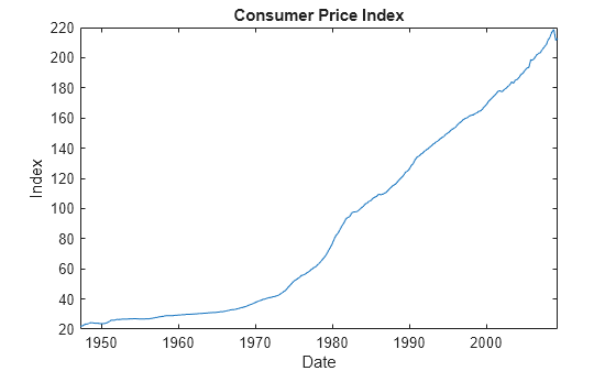
figure;
plot(DataTimeTable.Time,DataTimeTable.CPIAUCSL);
title('Consumer Price Index')
ylabel('Index')
xlabel('Date')
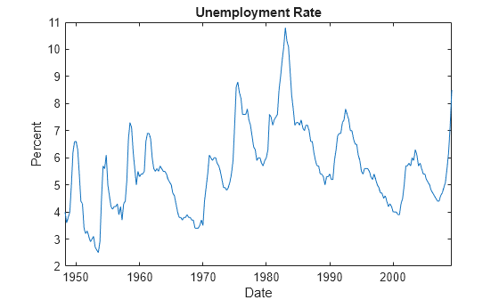
figure;
plot(DataTimeTable.Time,DataTimeTable.UNRATE);
title('Unemployment Rate');
ylabel('Percent');
xlabel('Date');
Stabilize the CPI by converting it to a series of growth rates. Synchronize the two series by removing the first observation from the unemployment rate series.
rcpi = price2ret(DataTimeTable.CPIAUCSL);
unrate = DataTimeTable.UNRATE(2:end);
Create a default VAR(4) model by using the shorthand syntax.
Mdl = varm(2,4)
Mdl =
  varm with properties:

     Description: "2-Dimensional VAR(4) Model"
     SeriesNames: "Y1"  "Y2"
       NumSeries: 2
               P: 4
        Constant: [2×1 vector of NaNs]
              AR: {2×2 matrices of NaNs} at lags [1 2 3 ... and 1 more]
           Trend: [2×1 vector of zeros]
            Beta: [2×0 matrix]
      Covariance: [2×2 matrix of NaNs]
Mdl is a varm model object. All properties containing NaN values correspond to parameters to be estimated given data.
Estimate the model using the entire data set.
EstMdl = estimate(Mdl,[rcpi unrate])
EstMdl =
  varm with properties:

     Description: "AR-Stationary 2-Dimensional VAR(4) Model"
     SeriesNames: "Y1"  "Y2"
       NumSeries: 2
               P: 4
        Constant: [0.00171639 0.316255]'
              AR: {2×2 matrices} at lags [1 2 3 ... and 1 more]
           Trend: [2×1 vector of zeros]
            Beta: [2×0 matrix]
      Covariance: [2×2 matrix]
EstMdl is an estimated varm model object. It is fully specified because all parameters have known values. The description indicates that the autoregressive polynomial is stationary.
Display summary statistics from the estimation.
summarize(EstMdl)
   AR-Stationary 2-Dimensional VAR(4) Model

    Effective Sample Size: 241
    Number of Estimated Parameters: 18
    LogLikelihood: 811.361
    AIC: -1586.72
    BIC: -1524

                      Value       StandardError    TStatistic      PValue
                   ___________    _____________    __________    __________

    Constant(1)      0.0017164      0.0015988         1.0735        0.28303
    Constant(2)        0.31626       0.091961          3.439      0.0005838
    AR{1}(1,1)         0.30899       0.063356          4.877     1.0772e-06
    AR{1}(2,1)         -4.4834         3.6441        -1.2303        0.21857
    AR{1}(1,2)      -0.0031796      0.0011306        -2.8122       0.004921
    AR{1}(2,2)          1.3433       0.065032         20.656      8.546e-95
    AR{2}(1,1)         0.22433       0.069631         3.2217      0.0012741
    AR{2}(2,1)          7.1896          4.005         1.7951       0.072631
    AR{2}(1,2)       0.0012375      0.0018631         0.6642        0.50656
    AR{2}(2,2)        -0.26817        0.10716        -2.5025       0.012331
    AR{3}(1,1)         0.35333       0.068287         5.1742     2.2887e-07
    AR{3}(2,1)           1.487         3.9277        0.37858          0.705
    AR{3}(1,2)       0.0028594      0.0018621         1.5355        0.12465
    AR{3}(2,2)        -0.22709         0.1071        -2.1202       0.033986
    AR{4}(1,1)       -0.047563       0.069026       -0.68906        0.49079
    AR{4}(2,1)          8.6379         3.9702         2.1757       0.029579
    AR{4}(1,2)     -0.00096323      0.0011142       -0.86448        0.38733
    AR{4}(2,2)        0.076725       0.064088         1.1972        0.23123


   Innovations Covariance Matrix:
    0.0000   -0.0002
   -0.0002    0.1167


   Innovations Correlation Matrix:
    1.0000   -0.0925
   -0.0925    1.0000
Fit a VAR(4) model to the consumer price index (CPI) and unemployment rate data. The estimation sample starts at Q1 of 1980.
Load the Data_USEconModel data set.
load Data_USEconModelStabilize the CPI by converting it to a series of growth rates. Synchronize the two series by removing the first observation from the unemployment rate series.
rcpi = price2ret(DataTimeTable.CPIAUCSL);
unrate = DataTimeTable.UNRATE(2:end);
Identify the index corresponding to the start of the estimation sample.
estIdx = DataTimeTable.Time(2:end) > '1979-12-31';Create a default VAR(4) model by using the shorthand syntax.
Mdl = varm(2,4);
Estimate the model using the estimation sample. Specify all observations before the estimation sample as presample data. Display a full estimation summary.
Y0 = [rcpi(~estIdx) unrate(~estIdx)];
EstMdl = estimate(Mdl,[rcpi(estIdx) unrate(estIdx)],'Y0',Y0,'Display',"full");
   AR-Stationary 2-Dimensional VAR(4) Model

    Effective Sample Size: 117
    Number of Estimated Parameters: 18
    LogLikelihood: 419.837
    AIC: -803.674
    BIC: -753.955

                     Value       StandardError    TStatistic      PValue
                   __________    _____________    __________    __________

    Constant(1)      0.003564      0.0024697         1.4431        0.14898
    Constant(2)       0.29922        0.11882         2.5182       0.011795
    AR{1}(1,1)       0.022379       0.092458        0.24204        0.80875
    AR{1}(2,1)        -2.6318         4.4484       -0.59163         0.5541
    AR{1}(1,2)     -0.0082357      0.0020373        -4.0425     5.2884e-05
    AR{1}(2,2)         1.2567        0.09802          12.82     1.2601e-37
    AR{2}(1,1)        0.20954        0.10182         2.0581       0.039584
    AR{2}(2,1)         10.106         4.8987          2.063       0.039117
    AR{2}(1,2)      0.0058667       0.003194         1.8368       0.066236
    AR{2}(2,2)       -0.14226        0.15367       -0.92571        0.35459
    AR{3}(1,1)        0.56095       0.098691         5.6839     1.3167e-08
    AR{3}(2,1)        0.44406         4.7483       0.093518        0.92549
    AR{3}(1,2)      0.0049062       0.003227         1.5204        0.12841
    AR{3}(2,2)      -0.040037        0.15526       -0.25787         0.7965
    AR{4}(1,1)       0.046125        0.11163        0.41321        0.67945
    AR{4}(2,1)          6.758         5.3707         1.2583        0.20827
    AR{4}(1,2)     -0.0030032       0.002018        -1.4882         0.1367
    AR{4}(2,2)       -0.14412       0.097094        -1.4843        0.13773


   Innovations Covariance Matrix:
    0.0000   -0.0003
   -0.0003    0.0790


   Innovations Correlation Matrix:
    1.0000   -0.1686
   -0.1686    1.0000
Because the VAR model degree p is 4, estimate uses only the last four observations in Y0 as a presample.
Since R2022b
Fit a VAR(4) model to the consumer price index (CPI) and unemployment rate series. Supply a timetable of data and specify the series for the fit.
Load and Preprocess Data
Load the Data_USEconModel data set. Compute the CPI growth rate. Because the growth rate calculation consumes the earliest observation, include the rate variable in the timetable by prepending the series with NaN.
load Data_USEconModel
DataTimeTable.RCPI = [NaN; price2ret(DataTimeTable.CPIAUCSL)];
numobs = height(DataTimeTable)
numobs = 249
Prepare Timetable for Estimation
When you plan to supply a timetable directly to estimate, you must ensure it has all the following characteristics:
All selected response variables are numeric and do not contain any missing values.
The timestamps in the
Timevariable are regular, and they are ascending or descending.
Remove all missing values from the table, relative to the CPI rate (RCPI) and unemployment rate (UNRATE) series.
varnames = ["RCPI" "UNRATE"];
DTT = rmmissing(DataTimeTable,DataVariables=varnames);
numobs = height(DTT)
numobs =
245
rmmissing removes the four initial missing observations from the DataTimeTable to create a sub-table DTT. The variables RCPI and UNRATE of DTT do not have any missing observations.
Determine whether the sampling timestamps have a regular frequency and are sorted.
areTimestampsRegular = isregular(DTT,"quarters")areTimestampsRegular = logical
0
areTimestampsSorted = issorted(DTT.Time)
areTimestampsSorted = logical
   1
areTimestampsRegular = 0 indicates that the timestamps of DTT are irregular. areTimestampsSorted = 1 indicates that the timestamps are sorted. Macroeconomic series in this example are timestamped at the end of the month. This quality induces an irregularly measured series.
Remedy the time irregularity by shifting all dates to the first day of the quarter.
dt = DTT.Time;
dt = dateshift(dt,"start","quarter");
DTT.Time = dt;
areTimestampsRegular = isregular(DTT,"quarters")
areTimestampsRegular = logical
   1
DTT is regular with respect to time.
Create Model Template for Estimation
Create a default VAR(4) model by using the shorthand syntax. Specify the response variable names.
Mdl = varm(2,4);
Mdl.SeriesNames = varnames
Mdl =
  varm with properties:

     Description: "2-Dimensional VAR(4) Model"
     SeriesNames: "RCPI"  "UNRATE"
       NumSeries: 2
               P: 4
        Constant: [2×1 vector of NaNs]
              AR: {2×2 matrices of NaNs} at lags [1 2 3 ... and 1 more]
           Trend: [2×1 vector of zeros]
            Beta: [2×0 matrix]
      Covariance: [2×2 matrix of NaNs]
Fit Model to Data
Estimate the model. Pass the entire timetable DTT. By default, estimate selects the response variables in Mdl.SeriesNames to fit to the model. Alternatively, you can use the ResponseVariables name-value argument.
Return the timetable of residuals and data fit to the model. Summarize the estimated model.
[EstMdl,~,~,Tbl2] = estimate(Mdl,DTT);
summarize(EstMdl)
   AR-Stationary 2-Dimensional VAR(4) Model

    Effective Sample Size: 241
    Number of Estimated Parameters: 18
    LogLikelihood: 811.361
    AIC: -1586.72
    BIC: -1524

                      Value       StandardError    TStatistic      PValue
                   ___________    _____________    __________    __________

    Constant(1)      0.0017164      0.0015988         1.0735        0.28303
    Constant(2)        0.31626       0.091961          3.439      0.0005838
    AR{1}(1,1)         0.30899       0.063356          4.877     1.0772e-06
    AR{1}(2,1)         -4.4834         3.6441        -1.2303        0.21857
    AR{1}(1,2)      -0.0031796      0.0011306        -2.8122       0.004921
    AR{1}(2,2)          1.3433       0.065032         20.656      8.546e-95
    AR{2}(1,1)         0.22433       0.069631         3.2217      0.0012741
    AR{2}(2,1)          7.1896          4.005         1.7951       0.072631
    AR{2}(1,2)       0.0012375      0.0018631         0.6642        0.50656
    AR{2}(2,2)        -0.26817        0.10716        -2.5025       0.012331
    AR{3}(1,1)         0.35333       0.068287         5.1742     2.2887e-07
    AR{3}(2,1)           1.487         3.9277        0.37858          0.705
    AR{3}(1,2)       0.0028594      0.0018621         1.5355        0.12465
    AR{3}(2,2)        -0.22709         0.1071        -2.1202       0.033986
    AR{4}(1,1)       -0.047563       0.069026       -0.68906        0.49079
    AR{4}(2,1)          8.6379         3.9702         2.1757       0.029579
    AR{4}(1,2)     -0.00096323      0.0011142       -0.86448        0.38733
    AR{4}(2,2)        0.076725       0.064088         1.1972        0.23123


   Innovations Covariance Matrix:
    0.0000   -0.0002
   -0.0002    0.1167


   Innovations Correlation Matrix:
    1.0000   -0.0925
   -0.0925    1.0000
EstMdl is an estimated varm model object. It is fully specified because all parameters have known values.
Display the head of the table Tbl2.
head(Tbl2)
    Time      COE     CPIAUCSL    FEDFUNDS    GCE      GDP     GDPDEF    GPDI    GS10    HOANBS    M1SL    M2SL    PCEC     TB3MS    UNRATE       RCPI       RCPI_Residuals    UNRATE_Residuals
    _____    _____    ________    ________    ____    _____    ______    ____    ____    ______    ____    ____    _____    _____    ______    __________    ______________    ________________

    Q1-49    144.1     23.91        NaN       45.6      270    16.531    40.9    NaN     53.961    NaN     NaN       177    1.17        5      -0.0058382      -0.013422             0.64674
    Q2-49    141.9     23.92        NaN       47.3    266.2     16.35      34    NaN     53.058    NaN     NaN     178.6    1.17      6.2      0.00041815      0.0051673              0.6439
    Q3-49      141     23.75        NaN       47.2    267.7    16.256    37.3    NaN     52.501    NaN     NaN       178    1.07      6.6      -0.0071324      0.0030175           -0.099092
    Q4-49    140.5     23.61        NaN       46.6    265.2    16.272    35.2    NaN     52.291    NaN     NaN     180.4     1.1      6.6      -0.0059122      -0.001196          -0.0066535
    Q1-50    144.6     23.64        NaN       45.6    275.2    16.222    44.4    NaN     52.696    NaN     NaN     183.1    1.12      6.3       0.0012698      0.0024607           -0.013354
    Q2-50    150.6     23.88        NaN       46.1    284.6    16.286    49.9    NaN     53.997    NaN     NaN       187    1.15      5.4        0.010101       0.010823            -0.53098
    Q3-50      159     24.34        NaN       45.9      302     16.63    56.1    NaN       55.7    NaN     NaN     200.7     1.3      4.4         0.01908       0.012566            -0.38177
    Q4-50    166.9     24.98        NaN       49.5    313.4     16.95    65.9    NaN     56.213    NaN     NaN     198.1    1.34      4.3        0.025954       0.010998             0.50761
Because the VAR model has degree of 4, estimation requires four presample observations. Consequently, estimate uses the first four rows (all quarters of 1948) of DTT as a presample, fits the model to the remaining observations, and returns only those observations used in estimation in Tbl2.
Plot the residuals.
figure
tiledlayout(2,1)
nexttile
plot(Tbl2.Time,Tbl2.RCPI_Residuals)
hold on
yline(0,"r--");
hold off
title("CPI Rate Residuals")
nexttile
plot(Tbl2.Time,Tbl2.UNRATE_Residuals)
hold on
yline(0,"r--");
hold off
title("Unemployment Rate Residuals")

Estimate a VAR(4) model of the consumer price index (CPI), unemployment rate, and real gross domestic product (GDP). Include a linear regression component containing the current quarter and the last four quarters of government consumption expenditures and investment (GCE).
Load the Data_USEconModel data set. Compute the real GDP.
load Data_USEconModel
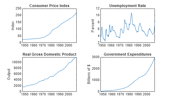
DataTimeTable.RGDP = DataTimeTable.GDP./DataTimeTable.GDPDEF*100;Plot all variables on separate plots.
figure
tiledlayout(2,2)
nexttile
plot(DataTimeTable.Time,DataTimeTable.CPIAUCSL);
ylabel('Index')
title('Consumer Price Index')
nexttile
plot(DataTimeTable.Time,DataTimeTable.UNRATE);
ylabel('Percent')
title('Unemployment Rate')
nexttile
plot(DataTimeTable.Time,DataTimeTable.RGDP);
ylabel('Output')
title('Real Gross Domestic Product')
nexttile
plot(DataTimeTable.Time,DataTimeTable.GCE);
ylabel('Billions of $')
title('Government Expenditures')
Stabilize the CPI, GDP, and GCE series by converting each to a series of growth rates. Synchronize the unemployment rate series with the others by removing its first observation.
inputVariables = {'CPIAUCSL' 'RGDP' 'GCE'};
Data = varfun(@price2ret,DataTimeTable,'InputVariables',inputVariables);
Data.Properties.VariableNames = inputVariables;
Data.UNRATE = DataTimeTable.UNRATE(2:end);
Expand the GCE rate series to a matrix that includes its current value and up through four lagged values. Remove the GCE variable from Data.
rgcelag4 = lagmatrix(Data.GCE,0:4);
Data.GCE = [];
Create a default VAR(4) model by using the shorthand syntax. You do not have to specify the regression component when creating the model.
Mdl = varm(3,4);
Estimate the model using the entire sample. Specify the GCE rate matrix as data for the regression component. Extract standard errors and the loglikelihood value.
[EstMdl,EstSE,logL] = estimate(Mdl,Data.Variables,'X',rgcelag4);Display the regression coefficient matrix.
EstMdl.Beta
ans = 3×5

    0.0777   -0.0892   -0.0685   -0.0181    0.0330
    0.1450   -0.0304    0.0579   -0.0559    0.0185
   -2.8138   -0.1636    0.3905    1.1799   -2.3328
EstMdl.Beta is a 3-by-5 matrix. Rows correspond to response series, and columns correspond to predictors.
Display the matrix of standard errors corresponding to the coefficient estimates.
EstSE.Beta
ans = 3×5

    0.0250    0.0272    0.0275    0.0274    0.0243
    0.0368    0.0401    0.0405    0.0403    0.0358
    1.4552    1.5841    1.6028    1.5918    1.4145
EstSE.Beta is commensurate with EstMdl.Beta.
Display the loglikelihood value.
logL
logL =
1.7056e+03
Input Arguments
Name-Value Arguments
Output Arguments
References
[1] Hamilton, James D. Time Series Analysis. Princeton, NJ: Princeton University Press, 1994.
[2] Johansen, S. Likelihood-Based Inference in Cointegrated Vector Autoregressive Models. Oxford: Oxford University Press, 1995.
[3] Juselius, K. The Cointegrated VAR Model. Oxford: Oxford University Press, 2006.
[4] Lütkepohl, H. New Introduction to Multiple Time Series Analysis. Berlin: Springer, 2005.