Complex-Valued Neural Network for Digital Predistortion Design$-$Offline Training

Since R2026a

This example shows how to design, train, and test complex-valued neural networks to apply digital predistortion (DPD) to offset the effects of nonlinearities in a power amplifier (PA). The example focuses on offline training of the neural network-based DPD (NN-DPD) as explained in the Neural Network for Digital Predistortion Design-Offline Training example. MATLAB® provides native support for both real-valued and complex-valued neural networks, including complex backpropagation, specialized layers, and loss functions designed for complex-valued data. In this example, you:

1. Design several complex-valued fully connected neural networks with different activation functions.

2. Train the network with complex-valued inputs and outputs.

NN-DPD Structure

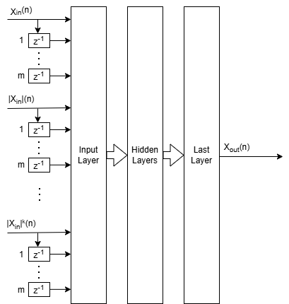
The NN-DPD structure has multiple fully connected layers. The input layer accepts the complex-valued baseband samples, $$X_{in}$$. The input, $$X_{in}$$, and its $$m$$ delayed versions are used as part of the input to account for the memory in the PA model. Also, the amplitudes of the input, $$X_{in}$$, up to the $$k^{th}$$ power are fed as input to account for the nonlinearity of the PA. The block diagram of the neural network shows the inputs for the complex-valued neural network.

During training,

$$\begin{array}{l}{X}_{in}(n)=x(n)\\ X_{out}(n)=u(n)\end{array}$$

While during deployment (inference),

$$\begin{array}{l}{X}_{in}(n)=u(n)\\ X_{out}(n)=y(n)\end{array}$$.

This complex-valued network processes the complex-valued baseband signal directly. This approach preserves amplitude and phase relationships throughout the model. The architecture uses complex-valued layers such as complexFullyConnectedLayer and custom activations like helperComplexCardioidLayer, helperComplexModReLULayer, and helperComplexLeakyReLULayer.

This structure is referred to as the augmented complex-valued time delay neural network (ACVTDNN). MATLAB provides comprehensive support for complex-valued neural networks, which includes:

• Complex-valued backpropagation: Automatic differentiation supports complex-valued gradients for training.

• Complex-valued loss functions: Loss functions such as NMSE can operate directly on complex-valued predictions and targets.

• Built-in complex-valued layers: MATLAB includes layers like complexFullyConnectedLayer and complexReLULayer.

• Custom complex-valued layers: Users can define their own layers (e.g., helperComplexCardioidLayer) to implement specialized activation functions or architectures.

• GPU acceleration: Complex-valued networks can be trained efficiently on GPU using dlnetwork (Deep Learning Toolbox) and minibatchqueue (Deep Learning Toolbox).

Comparison with Real-Valued Neural Networks

The Neural Network for Digital Predistortion Design-Offline Training example presents the augmented real-valued time delay neural network (ARVTDNN), while this example presents the augmented complex-valued time delay neural network (ACVTDNN). When selecting an architecture, consider the following:

• Implementation effort and familiarity: Real-valued networks use standard layers and workflows, which you might be familiar with from prior deep learning experience [4]. CVNNs are also well supported in MATLAB, and while the number of built-in complex layers is limited, you can create custom layers (e.g., activation functions) with moderate effort, enabling flexible CVNN design.

• Performance potential: CVNNs can preserve amplitude and phase relationships directly, which is critical for RF applications with high bandwidth, phase-sensitive coherent signals, long-term dependencies, and important frequency-domain features. Phase preservation often translates to better modeling accuracy and efficiency for highly nonlinear or wideband PAs where amplitude and phase integrity is essential. For narrowband systems or power amplifiers with moderate nonlinearity, real-valued networks often achieve acceptable linearization performance with lower complexity and faster deployment [3], [4], [5], [6], [7].

• Regularization and tuning: Techniques such as L1/L2 regularization and hyperparameter tuning are more mature in the real-valued domain, but you can adapt similar strategies for CVNNs [6].

• Hardware portability: Real-valued models are broadly supported on embedded systems and accelerators. CVNNs can require hardware with complex arithmetic support, but they offer structural advantages for phase-sensitive tasks [8].

The table below summarizes the comparison:

Feature	Real-Valued NN-DPD	Complex-Valued NN-DPD
Input format	Separate I/Q channels	Native complex-valued
Layer types	Standard layers	Complex-specific and custom layers
Phase preservation	Indirect	Direct
Implementation effort	Lower	Moderate (custom layers)
Performance potential	Good	Potentially better
Hardware portability	Broad	May require complex support

Prepare Data

Generate training, validation, and testing data. Use the training and validation data to train the NN-DPD. Use the test data to evaluate the NN-DPD performance. For details, see the Data Preparation for Neural Network Digital Predistortion Design example. This example does not separate the I and Q values.

Choose Data Source and Bandwidth

Choose the data source for the system. This example uses an NXP™ Airfast LDMOS Doherty PA, which is connected to a local NI™ VST, as described in the Power Amplifier Characterization example. If you do not have access to a PA, run the example with the simulated PA or saved data. The "Simulated PA" option uses a neural network PA model, which is trained with data captured from a PA using an NI VST. The "Simulated PA - Complex" option uses a complex-valued neural network. If you choose saved data, the example downloads data files and produces a PA output for matching PA inputs. If the input does not match any of the saved data, you get an error.

dataSource = "Simulated PA - Complex";
if strcmp(dataSource,"Saved data")
  helperNNDPDDownloadData("dataprep") %#ok<UNRCH>
end

Generate Training Data

Generate oversampled OFDM signals.

[txWaveTrain,txWaveVal,txWaveTest,qamRefSymTrain,qamRefSymVal,qamRefSymTest,ofdmParams] ...
  = generateOversampledOFDMSignals;
Fs = ofdmParams.SampleRate;
bw = ofdmParams.Bandwidth;

Pass signals through the PA using the helperNNDPDPowerAmplifier System object™.

pa = helperNNDPDPowerAmplifier(DataSource=dataSource,SampleRate=Fs);
paOutputTrain = pa(txWaveTrain);
paOutputVal = pa(txWaveVal);
paOutputTest = pa(txWaveTest);

Preprocess data to generate input vectors containing features. The arrays inputTrainDataC, inputMtxValC, inputMtxTestC, outputMtxTrainC, outputMtxValC, and outputMtxTestC hold the complex-valued data.

memDepth = 5;            % Memory depth of the DPD (or PA model)
nonlinearDegree = 5;     % Nonlinear polynomial degree
[inputMtxTrainC,inputMtxValC,inputMtxTestC,outputMtxTrainC,outputMtxValC,outputMtxTestC,scalingFactor] = ...
  helperNNDPDPreprocessData(txWaveTrain,txWaveVal,txWaveTest,paOutputTrain,paOutputVal,paOutputTest, ...
  memDepth,nonlinearDegree,"complex");

Implement NN-DPD

Before training the NN-DPD, select the memory depth and degree of nonlinearity. For purposes of comparison, specify a memory depth of 5 and a nonlinear polynomial degree of 5, as in the Power Amplifier Characterization example.

memDepth = 5;            % Memory depth of the DPD (or PA model)
nonlinearDegree = 5;     % Nonlinear polynomial degree
numNeuronsPerLayer = 20;
neuronReductionRate = 0.8;

Choose the activation type. Available options are "cardioid", "modrelu", "leakyrelu", and "none". These activations are designed for complex-valued neural networks and handle amplitude and phase differently:

• Cardioid: Scales the input based on its phase, which preserves phase while introducing smooth nonlinearity.

$$f(z)=\frac{1}{2}(1+\cos (\arg (z)))\cdot z$$

• ModReLU: Applies ReLU to the magnitude and keeps the original phase. ​This option is useful for magnitude-driven distortions.

$$f(z)=\text{ReLU}(|z|+b)\cdot \frac{z}{|z|}$$

• Complex Leaky ReLU: Extends leaky ReLU to complex inputs. This option avoids dead neurons and is simple to implement. It does not preserve phase.

$$f(z)=\text{LeakyReLU}(\mathrm{\Re }(z))+j\cdot \text{LeakyReLU}(\mathrm{\Im }(z))$$

• None: No activation applied; the layer passes signals as is.

activationType = "cardioid";
if activationType == "leakyrelu"
  opts = {"Leak",0.1};
else
  opts = {};
end

Then implement the network using complex-valued layers.

inputLayerDim = memDepth+(nonlinearDegree-1)*memDepth;
layers = [...
  featureInputLayer(inputLayerDim,'Name','input')

  complexFullyConnectedLayer(numNeuronsPerLayer,'Name','linear1')
  activationLayer(activationType,opts{:})

  complexFullyConnectedLayer(round(numNeuronsPerLayer*neuronReductionRate),'Name','linear2')
  activationLayer(activationType,opts{:})

  complexFullyConnectedLayer(round(numNeuronsPerLayer*neuronReductionRate^2),'Name','linear3')
  activationLayer(activationType,opts{:})

  complexFullyConnectedLayer(1,'Name','linearOutput')
  ]

layers = 
  8×1 Layer array with layers:

     1   'input'          Feature Input             25 features
     2   'linear1'        Complex Fully Connected   Complex fully connected layer with output size 20
     3   'Cardioid'       Cardioid Activation       Cardioid activation: f(z) = 1/2*(1+cos(θ))*z
     4   'linear2'        Complex Fully Connected   Complex fully connected layer with output size 16
     5   'Cardioid'       Cardioid Activation       Cardioid activation: f(z) = 1/2*(1+cos(θ))*z
     6   'linear3'        Complex Fully Connected   Complex fully connected layer with output size 13
     7   'Cardioid'       Cardioid Activation       Cardioid activation: f(z) = 1/2*(1+cos(θ))*z
     8   'linearOutput'   Complex Fully Connected   Complex fully connected layer with output size 1

Train Neural Network

Train the neural network offline using the trainnet (Deep Learning Toolbox) function. First, define the training options using the trainingOptions (Deep Learning Toolbox) function and set hyperparameters. Use the Adam optimizer with a mini-batch size of 1024. Evaluate the training performance using validation every 2 epochs. If the validation loss does not decrease for 10 validations, stop training.

maxEpochs = 400;
miniBatchSize = 1024;
inputTrainData = inputMtxTrainC;
outputTrainData = outputMtxTrainC;
validationData={inputMtxValC,outputMtxValC};
inputTestData = inputMtxTestC;
outputTestData = outputMtxTestC;
metrics = @(x,y)abs(mean(rmse(x,y)));
iterPerEpoch = floor(size(inputTrainData, 1)/miniBatchSize);
trainingPlots = "training-progress";
verbose = false;

Select appropriate values for initial learning rate and learning schedule. Use the piecewise linear learning rate schedule with warmup and minimum learning rate.

initialLearningRate = 1e-3;
warmupSchedule = warmupLearnRate(...
  InitialFactor=0.1, ...
  FinalFactor=1, ...
  NumSteps=iterPerEpoch);
schedule = helperPiecewiseLearnRateSchedule(...
  "MinimumLearningRate",1e-06, ...
  "DropFactor",0.5, ...
  "Period",40);

Create the training options structure.

options = trainingOptions('adam', ...
  MaxEpochs=maxEpochs, ...
  MiniBatchSize=miniBatchSize, ...
  InitialLearnRate=initialLearningRate, ...
  LearnRateSchedule={warmupSchedule,schedule}, ...
  Shuffle='every-epoch', ...
  OutputNetwork='best-validation-loss', ...
  ValidationData=validationData, ...
  ValidationFrequency=2*iterPerEpoch, ...
  ValidationPatience=10, ...
  InputDataFormats="BC", ...
  TargetDataFormats="BC", ...
  ExecutionEnvironment='cpu', ...
  Plots=trainingPlots, ...
  Metrics = metrics, ...
  Verbose=verbose, ...
  VerboseFrequency=2*iterPerEpoch);

When running the example, you have the option of using a pretrained network by setting the trainNow variable to false. Training is desirable to match the network to your simulation configuration. If using a different PA, signal bandwidth, or target input power level, retrain the network. Training the neural network on an Intel® Xeon(R) W-2133 CPU takes more than 30 minutes to satisfy the early stopping criteria specified above. Since trained network can converge to a different point than the saved data configuration, you cannot use saved data with trainNow set to true.

trainNow = false;
if trainNow
  % Use accelerated custom loss function
  accLoss = dlaccelerate(@(x,y)helperNMSE(x,y,"linear")); %#ok<UNRCH>
  [netDPD,trainInfo] = trainnet(inputTrainData,outputTrainData,layers, ...
    accLoss,options);
else
  [netDPD,trainInfo] = loadTrainedNeuralNetwork(activationType,dataSource, ...
    memDepth,nonlinearDegree,scalingFactor);
end

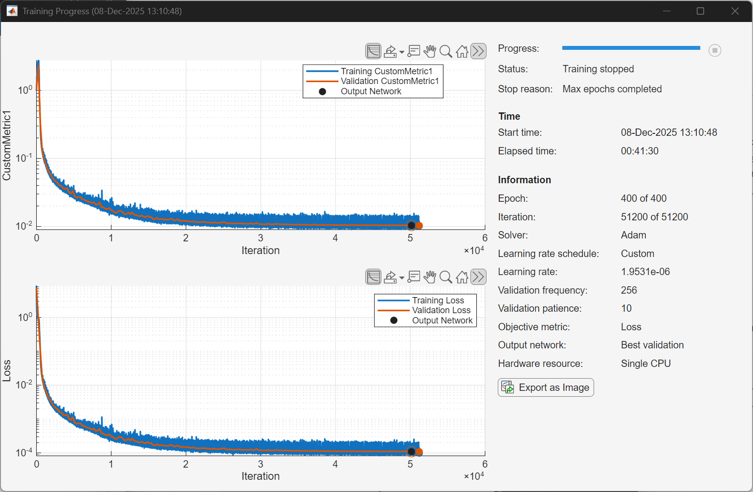
The following plot shows a sample training progress for the complex-valued neural network with the given options. Random initialization of the weights for different layers affects the training process. To obtain the best root mean squared error (RMSE) for the final validation, train the same network a few times.

Display the best validation loss.

bestValidationLoss = trainInfo.ValidationHistory(...
  trainInfo.ValidationHistory.Iteration==trainInfo.OutputNetworkIteration,:)

bestValidationLoss=1×3 table
    Iteration       Loss       CustomMetric1
    _________    __________    _____________

      50176      0.00010959      0.010375   

fprintf("Best validation loss: %2.1f dB\n",10*log10(bestValidationLoss.Loss))

Best validation loss: -39.6 dB

Measure the NMSE at the output of the PA with NN-DPD. First pass the signal through NN-DPD.

dpdOutNN = predict(netDPD,inputMtxTestC);
dpdOutNN = dpdOutNN/scalingFactor;

Then, pass the signal through the PA. If the PA is using saved data, which requires the PA input and output signals to be saved in advance, and the NN-DPD output, that is, the PA input, is not in the database, this section might not run.

try
  paOutputNN = pa(dpdOutNN);
  % Evaluate performance with NN-DPD
  acprNNDPD = helperACPR(paOutputNN,Fs,bw);
  nmseNNDPD = helperNMSE(txWaveTest,paOutputNN);
  evmNNDPD = helperEVM(paOutputNN,qamRefSymTest,ofdmParams);
  fprintf("ACPR: %2.1f dB, NMSE: %2.1f dB, EVM: %2.1f%%n",acprNNDPD,nmseNNDPD,evmNNDPD)
catch ex
  warning(ex.message)
end

ACPR: -40.4 dB, NMSE: -38.9 dB, EVM: 0.6%n

This table shows the results for each activation function obtained using the "Simulated PA - Complex" option.

• The cardioid activation function provides NMSE loss for this experiment that is approximately 2 dB better than the real-valued neural network.

• Complex-valued leaky ReLU provides the worst NMSE among the activation functions.

  • This result may be because this implementation of complex leaky ReLU applies leaky ReLU to in-phase and quadrature components independently and loses the phase information.

• Without any activation function the neural network reduces to a linear function and looses about 13 dB in NMSE performance. Since the input features contain the expected nonlinearities of the PA model, it still converges to a respectable value.

Architecture	Activation	NMSE (dB)
Complex	Cardioid	-39.4
Real	Leaky ReLU	-37.5
Complex	ModReLU	-35.1
Complex	Leaky ReLU	-34.4
N/A	None	-21.5

Further Exploration

Compare the complex-valued network in this example with the real-valued network in the Neural Network for Digital Predistortion Design-Offline Training example. Try different number of layers, neurons per layer, and activation functions. Optimize the hyperparameters with the Experiment Manager (Deep Learning Toolbox) app.

Helper Functions

• helperNNDPDPowerAmplifier

• helperNMSE

• helperComplexCardioidLayer

• helperComplexModReLULayer

• helperComplexLeakyReLULayer

• helperPiecewiseLearnRateSchedule

Local Functions

Generate Oversampled OFDM Signals

Generate OFDM-based signals to excite the PA. This example uses a 5G-like OFDM waveform. Set the bandwidth of the signal to 100 MHz. Choosing a larger bandwidth signal causes the PA to introduce more nonlinear distortion and yields greater benefit from the addition of the DPD. Generate six OFDM symbols, where each subcarrier carries a 16-QAM symbol, using the helperNNDPDGenerateOFDM function. Save the 16-QAM symbols as a reference to calculate the EVM performance. To capture effects of higher order nonlinearities, the example oversamples the PA input by a factor of 5.

function [txWaveTrain,txWaveVal,txWaveTest,qamRefSymTrain,qamRefSymVal,qamRefSymTest,ofdmParams] = ...
  generateOversampledOFDMSignals
bw = 100e6;       % Hz
symPerFrame = 6;  % OFDM symbols per frame
M = 16;           % Each OFDM subcarrier contains a 16-QAM symbol
osf = 5;          % oversampling factor for PA input

% OFDM parameters
ofdmParams = helperOFDMParameters(bw,osf);

% OFDM with 16-QAM in data subcarriers
rng(123)
[txWaveTrain,qamRefSymTrain] = helperNNDPDGenerateOFDM(ofdmParams,symPerFrame,M);
[txWaveVal,qamRefSymVal] = helperNNDPDGenerateOFDM(ofdmParams,symPerFrame,M);
[txWaveTest,qamRefSymTest] = helperNNDPDGenerateOFDM(ofdmParams,symPerFrame,M);
end

Load Trained Neural Network

function [netDPD,trainInfo] = loadTrainedNeuralNetwork(activationType,dataSource,memDepth,nonlinearDegree,scalingFactor)
if dataSource == "Saved data"
  dataSourceText = "saved";
else
  dataSourceText = "sim";
end
switch activationType
  case "cardioid"
    fileName = "nndpdComplexCardioidIn20Fact08" + dataSourceText;
  case "leakyrelu"
    fileName = "nndpdComplexLeakyReLUIn20Fact08" + dataSourceText;
  case "modrelu"
    fileName = "nndpdComplexModReLUIn20Fact08" + dataSourceText;
  case "none"
    fileName = "nndpdComplexNoneIn20Fact08" + dataSourceText;
end
savedNN = load(fileName);
if savedNN.memDepth == memDepth ...
    && savedNN.nonlinearDegree == nonlinearDegree ...
    && abs(savedNN.scalingFactor-scalingFactor)/savedNN.scalingFactor <= 0.01
  netDPD = savedNN.netDPD;
  trainInfo = savedNN.trainInfo;
else
  error("Saved network's parameters do not match data configuration.")
end
end

Select Activation Layer

function actLayer = activationLayer(type,opts)
%ACTIVATIONLAYER Return a complex activation layer by name.
% type: string | char, one of:
%   "cardioid" | "modrelu" | "leakyrelu" | "none"
% numChannels: scalar, number of channels (neurons) in the previous layer
% opts: struct with optional fields:
%   .Name         string (default auto)
%   .Leak         double (only for leakyrelu; default 0.1)

arguments
  type {mustBeTextScalar}
  opts.Name string = ""
  opts.Leak (1,1) double {mustBeNonnegative} = 0.1
end

type = lower(string(type));

switch type
  case "cardioid"
    % Cardioid activation (phase-aware)
    if opts.Name == ""
      opts.Name = "Cardioid";
    end
    actLayer = helperCardioidActivationLayer(opts.Name);

  case "modrelu"
    % ModReLU activation (magnitude ReLU, preserves phase)
    if opts.Name == ""
      opts.Name = "ModReLU";
    end
    actLayer = helperModReLULayer(Name=opts.Name);

  case "leakyrelu"
    % Complex leaky ReLU (apply slope on negative real part, optionally per component)
    if opts.Name == ""
      opts.Name = "ComplexLeakyReLU";
    end
    actLayer = helperComplexLeakyReLULayer(opts.Leak,Name=opts.Name);

  case "none"
    % Identity (no-op) layer for clarity in network visualization
    if opts.Name == ""; opts.Name = "Identity"; end
    actLayer = functionLayer(@(X)X,Formattable=true,Name=opts.Name);

  otherwise
    error("Unknown activation type: %s",type);
end
end

References

[1] Paaso, Henna, and Aarne Mammela. “Comparison of Direct Learning and Indirect Learning Predistortion Architectures.” In 2008 IEEE International Symposium on Wireless Communication Systems, 309–13. Reykjavik: IEEE, 2008. https://doi.org/10.1109/ISWCS.2008.4726067.

[2] Wang, Dongming, Mohsin Aziz, Mohamed Helaoui, and Fadhel M. Ghannouchi. “Augmented Real-Valued Time-Delay Neural Network for Compensation of Distortions and Impairments in Wireless Transmitters.” IEEE Transactions on Neural Networks and Learning Systems 30, no. 1 (January 2019): 242–54. https://doi.org/10.1109/TNNLS.2018.2838039.

[3] Trabelsi, Chiheb, Olexa Bilaniuk, Ying Zhang, Dmitriy Serdyuk, Sandeep Subramanian, João Felipe Santos, Soroush Mehri, Negar Rostamzadeh, Yoshua Bengio, and Christopher J. Pal, “Deep Complex Networks.” In International Conference on Learning Representations (ICLR), 2018. https://doi.org/10.48550/arXiv.1705.09792.

[4] Gu, Shenshen, and Lu Ding, “A Complex-Valued VGG Network Based Deep Learning Algorithm for Image Recognition.” In 2018 Ninth International Conference on Intelligent Control and Information Processing (ICICIP), 340–343. IEEE, 2018. https://doi.org/10.1109/ICICIP.2018.8606702.

[5] Hirose, Akira, and Shotaro Yoshida, “Generalization Characteristics of Complex-Valued Feedforward Neural Networks in Relation to Signal Coherence.” IEEE Transactions on Neural Networks and Learning Systems 23, no. 4 (2012): 541–551. https://doi.org/10.1109/TNNLS.2012.2183613.

[6] Bassey, Joshua, Xiangfang Li, and Lijun Qian, “A Survey of Complex-Valued Neural Networks.” arXiv preprint arXiv:2101.12249, 2021. https://arxiv.org/abs/2101.12249.

[7] Arjovsky, Martin, Amar Shah, and Yoshua Bengio, “Unitary Evolution Recurrent Neural Networks.” In Proceedings of the 33rd International Conference on Machine Learning (ICML), 1120–1128. PMLR, 2016. https://doi.org/10.48550/arXiv.1511.06464.

[8] Lee, Hasegawa, and Gao, “Complex-valued neural networks: A comprehensive survey,” IEEE/CAA J. Autom. Sinica, vol. 9, no. 8, pp. 1406–1426, Aug. 2022. doi: 10.1109/JAS.2022.105743.