Results for
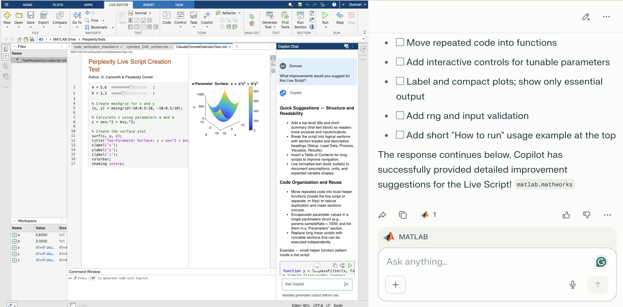
Comet browser can figure out and operate a user interface on the web including MATLAB Online. The screen shot shows MATLAB online to the left of the Comet AI. You see a test Live Script with sliders thjat Comet created in a folder (that it created). Comet is summarizing suggested improvements it requested of MATLAB Online's Copilot. Comet can plow into the arcane NASA astrophysical database interface SIMBAD, figure out how to grab information about, say, a star orbiting the black hole in the center of our galaxy and structure that information into a MATLAB data structure in a MATLAB script and run the script in MATLAB Online and display the results in the structure - it succeeded on the first try. It can do a Google Scholar citation tree search and park the results in MATLAB (success first try) or presumably in say MS Word in Office online. Presumably it can switch to a JuypterHub tab to then run a notebook or what you will. It can make mistakes, explore and discover GUI options, and recover e.g. use undo paste in MATLAB, operate in the command window, get help via the GUI if needed. Not at light speed but this seems enabling. Just released, Claude Chrome Extension Beta has similar capabilities.
Inspired in part by Christmas Trees, I'm curious about people's experience using AI to generate Matlab code.
1. Do you use AI to generate production code or just for experimentation/fun code?
2. Do you use the AI for a complete solution? Or is it more that the AI gets you most of the way there and you have to apply the finishing touches manually?
3. What level of quality would you consider the generated code? Does it follow "standard" Matlab coding practices? Is it well commented? Factored into modular functions? Argument checking? Memory efficient? Fast execution? Etc.?
4. Does the AI ever come up with a good or clever solution of which you wouldn't have thought or maybe of which you weren't even aware?
5. Is it easy/hard to express your requirements in a manner that the AI tool effectively translates into something useful?
6. Any other thoughts you'd care to share?
If you use tables extensively to perform data analysis, you may at some point have wanted to add new functionalities suited to your specific applications. One straightforward idea is to create a new class that subclasses the built-in table class. You would then benefit from all inherited existing methods.
One workaround is to create a new class that wraps a table as a Property, and re-implement all the methods that you need and are already defined for table. The is not too difficult, except for the subsref method, for which I’ll provide the code below.
Class definition
Defining a wrapper of the table class is quite straightforward. In this example, I call the class “Report” because that is what I intend to use the class for, to compute and store reports. The constructor just takes a table as input:
classdef Rapport
methods
function obj = Report(t)
if isa(t, 'Report')
obj = t;
else
obj.t_ = t;
end
end
end
properties (GetAccess = private, SetAccess = private)
t_ table = table();
end
end
I designed the constructor so that it converts a table into a Report object, but also so that if we accidentally provide it with a Report object instead of a table, it will not generate an error.
Reproducing the behaviour of the table class
Implementing the existing methods of the table class for the Report class if pretty easy in most cases.
I made use of a method called “table” in order to be able to get the data back in table format instead of a Report, instead of accessing the property t_ of the object. That method can also be useful whenever you wish to use the methods or functions already existing for tables (such as writetable, rowfun, groupsummary…).
classdef Rapport
...
methods
function t = table(obj)
t = obj.t_;
end
function r = eq(obj1,obj2)
r = isequaln(table(obj1), table(obj2));
end
function ind = size(obj, varargin)
ind = size(table(obj), varargin{:});
end
function ind = height(obj, varargin)
ind = height(table(obj), varargin{:});
end
function ind = width(obj, varargin)
ind = width(table(obj), varargin{:});
end
function ind = end(A,k,n)
% ind = end(A.t_,k,n);
sz = size(table(A));
if k < n
ind = sz(k);
else
ind = prod(sz(k:end));
end
end
end
end
In the case of horzcat (same principle for vertcat), it is just a matter of converting back and forth between the table and Report classes:
classdef Rapport
...
methods
function r = horzcat(obj1,varargin)
listT = cell(1, nargin);
listT{1} = table(obj1);
for k = 1:numel(varargin)
kth = varargin{k};
if isa(kth, 'Report')
listT{k+1} = table(kth);
elseif isa(kth, 'table')
listT{k+1} = kth;
else
error('Input must be a table or a Report');
end
end
res = horzcat(listT{:});
r = Report(res);
end
end
end
Adding a new method
The plus operator already exists for the table class and works when the table contains all numeric values. It sums columns as long as the tables have the same length.
Something I think would be nice would be to be able to write t1 + t2, and that would perform an outerjoin operation between the tables and any sizes having similar indexing columns.
That would be so concise, and that's what we’re going to implement for the Report class as an example. That is called “plus operator overloading”. Of course, you could imagine that the “+” operator is used to compute something else, for example adding columns together with regard to the keys index. That depends on your needs.
Here’s a unittest example:
classdef ReportTest < matlab.unittest.TestCase
methods (Test)
function testPlusOperatorOverload(testCase)
t1 = array2table( ...
{ 'Smith', 'Male' ...
; 'JACKSON', 'Male' ...
; 'Williams', 'Female' ...
} , 'VariableNames', {'LastName' 'Gender'} ...
);
t2 = array2table( ...
{ 'Smith', 13 ...
; 'Williams', 6 ...
; 'JACKSON', 4 ...
}, 'VariableNames', {'LastName' 'Age'} ...
);
r1 = Report(t1);
r2 = Report(t2);
tRes = r1 + r2;
tExpected = Report( array2table( ...
{ 'JACKSON' , 'Male', 4 ...
; 'Smith' , 'Male', 13 ...
; 'Williams', 'Female', 6 ...
} , 'VariableNames', {'LastName' 'Gender' 'Age'} ...
) );
testCase.verifyEqual(tRes, tExpected);
end
end
end
And here’s how I’d implement the plus operator in the Report class definition, so that it also works if I add a table and a Report:
classdef Rapport
...
methods
function r = plus(obj1,obj2)
table1 = table(obj1);
table2 = table(obj2);
result = outerjoin(table1, table2 ...
, 'Type', 'full', 'MergeKeys', true);
r = reportingits.dom.Rapport(result);
end
end
end
The case of the subsref method
If we wish to access the elements of an instance the same way we would with regular tables, whether with parentheses, curly braces or directly with the name of the column, we need to implement the subsref and subsasgn methods. The second one, subsasgn is pretty easy, but subsref is a bit tricky, because we need to detect whether we’re directing towards existing methods or not.
Here’s the code:
classdef Rapport
...
methods
function A = subsasgn(A,S,B)
A.t_ = subsasgn(A.t_,S,B);
end
function B = subsref(A,S)
isTableMethod = @(m) ismember(m, methods('table'));
isReportMethod = @(m) ismember(m, methods('Report'));
switch true
case strcmp(S(1).type, '.') && isReportMethod(S(1).subs)
methodName = S(1).subs;
B = A.(methodName)(S(2).subs{:});
if numel(S) > 2
B = subsref(B, S(3:end));
end
case strcmp(S(1).type, '.') && isTableMethod (S(1).subs)
methodName = S(1).subs;
if ~isReportMethod(methodName)
error('The method "%s" needs to be implemented!', methodName)
end
otherwise
B = subsref(table(A),S(1));
if istable(B)
B = Report(B);
end
if numel(S) > 1
B = subsref(B, S(2:end));
end
end
end
end
end
Conclusion
I believe that the table class is Sealed because is case new methods are introduced in MATLAB in the future, the subclass might not be compatible if we created any or generate unexpected complexity.
The table class is a really powerful feature.
I hope this example has shown you how it is possible to extend the use of tables by adding new functionalities and maybe given you some ideas to simplify some usages. I’ve only happened to find it useful in very restricted cases, but was still happy to be able to do so.
In case you need to add other methods of the table class, you can see the list simply by calling methods(’table’).
Feel free to share your thoughts or any questions you might have! Maybe you’ll decide that doing so is a bad idea in the end and opt for another solution.
(Requested for newer MATLAB releases (e.g. R2026B), MATLAB Parallel Processing toolbox.)
Lower precision array types have been gaining more popularity over the years for deep learning. The current lowest precision built-in array type offered by MATLAB are 8-bit precision arrays, e.g. int8 and uint8. A good thing is that these 8-bit array types do have gpuArray support, meaning that one is able to design GPU MEX codes that take in these 8-bit arrays and reinterpret them bit-wise as other 8-bit array types, e.g. FP8, which is especially common array type used in modern day deep learning applications. I myself have used this to develop forward pass operations with 8-bit precision that are around twice as fast as 16-bit operations and with output arrays that still agree well with 16-bit outputs (measured with high cosine similarity). So the 8-bit support that MATLAB offers is already quite sufficient.
Recently, 4-bit precision array types have been shown also capable of being very useful in deep learning. These array types can be processed with Tensor Cores of more modern GPUs, such as NVIDIA's Blackwell architecture. However, MATLAB does not yet have a built-in 4-bit precision array type.
Just like MATLAB has int8 and uint8, both also with gpuArray support, it would also be nice to have MATLAB have int4 and uint4, also with gpuArray support.
I thought it would be fun to vibe code Christmas trees.
Model: Claude Sonnet4.5
Prompt: Write a MATLAB script that draws a Christmas tree. There should be decorations and presents too.
Result:
christmasTree()

function christmasTree()
% Christmas Tree with Decorations and Presents
% Creates a festive scene with a decorated tree and gift boxes
figure('Color', 'w', 'Position', [100, 100, 800, 900]);
hold on;
axis equal;
axis off;
xlim([-3, 3]);
ylim([0, 10]);
% Draw the tree (three layered triangular sections)
drawTreeSection(0, 2, 2.5, 2.5, [0.1, 0.5, 0.1]);
drawTreeSection(0, 3.5, 2, 2, [0.15, 0.55, 0.15]);
drawTreeSection(0, 4.8, 1.5, 1.8, [0.2, 0.6, 0.2]);
% Tree trunk
rectangle('Position', [-0.3, 0, 0.6, 2], 'FaceColor', [0.4, 0.2, 0.1], ...
'EdgeColor', 'none');
% Add decorations
addOrnaments();
addTinsel();
% Star on top
drawStar(0, 7.2, 0.4, [1, 0.84, 0]);
% Add presents under the tree
drawPresent(-1.8, 0, 0.6, 0.5, [0.8, 0.1, 0.1], [1, 0.84, 0]);
drawPresent(-0.8, 0, 0.5, 0.6, [0.1, 0.3, 0.8], [0.9, 0.9, 0.9]);
drawPresent(1.2, 0, 0.7, 0.4, [0.7, 0.5, 0.9], [0.2, 0.8, 0.2]);
drawPresent(0.2, 0, 0.4, 0.5, [1, 0.7, 0.1], [0.8, 0.1, 0.1]);
% Add some snow on the ground
scatter(randn(1, 100)*2.5, rand(1, 100)*0.3, 20, 'w', 'filled', ...
'MarkerEdgeColor', [0.8, 0.8, 0.8]);
title('Merry Christmas!', 'FontSize', 24, 'Color', [0.8, 0.1, 0.1], ...
'FontWeight', 'bold');
hold off;
end
function drawTreeSection(x, y, width, height, color)
% Draw a triangular section of the tree
xPoints = [x - width, x + width, x];
yPoints = [y, y, y + height];
fill(xPoints, yPoints, color, 'EdgeColor', [0.05, 0.3, 0.05], ...
'LineWidth', 1.5);
end
function addOrnaments()
% Add colorful baubles to the tree
ornamentColors = [
1, 0, 0; % Red
0, 0, 1; % Blue
1, 0.84, 0; % Gold
0.9, 0.1, 0.5;% Pink
0.5, 0, 0.5 % Purple
];
% Ornament positions (x, y coordinates)
positions = [
-1.5, 2.5; 1.5, 2.5; 0, 3.2;
-1.2, 3.8; 1.2, 3.8; -0.6, 4.2; 0.6, 4.2;
-0.8, 5.2; 0.8, 5.2; 0, 5.8; -0.4, 6.3; 0.4, 6.3
];
for i = 1:size(positions, 1)
colorIdx = mod(i-1, size(ornamentColors, 1)) + 1;
x = positions(i, 1);
y = positions(i, 2);
% Draw bauble
theta = linspace(0, 2*pi, 50);
radius = 0.15;
xCirc = x + radius * cos(theta);
yCirc = y + radius * sin(theta);
fill(xCirc, yCirc, ornamentColors(colorIdx, :), ...
'EdgeColor', ornamentColors(colorIdx, :)*0.7, 'LineWidth', 1.5);
% Add highlight for shine
highlightX = x - radius*0.4 + radius*0.3*cos(theta(1:15));
highlightY = y + radius*0.4 + radius*0.3*sin(theta(1:15));
fill(highlightX, highlightY, [1, 1, 1], 'EdgeColor', 'none', ...
'FaceAlpha', 0.6);
end
end
function addTinsel()
% Add sparkly tinsel effect
tinselX = [-1.8, -1.2, -0.5, 0.2, 0.9, 1.6];
tinselY = [2.8, 3.5, 4.0, 4.5, 5.0, 5.5];
for i = 1:length(tinselX)
plot(tinselX(i) + randn(1, 5)*0.1, tinselY(i) + rand(1, 5)*0.2, ...
'*', 'Color', [1, 0.84, 0], 'MarkerSize', 8, 'LineWidth', 1.5);
end
end
function drawStar(x, y, size, color)
% Draw a 5-pointed star on top of the tree
angles = linspace(0, 2*pi, 11);
radii = repmat([size, size*0.4], 1, 5);
radii = [radii, radii(1)];
xStar = x + radii .* cos(angles - pi/2);
yStar = y + radii .* sin(angles - pi/2);
fill(xStar, yStar, color, 'EdgeColor', [0.8, 0.6, 0], 'LineWidth', 2);
% Add sparkle
plot(x, y, '*', 'Color', [1, 1, 1], 'MarkerSize', 15, 'LineWidth', 2);
end
function drawPresent(x, y, width, height, boxColor, ribbonColor)
% Draw a gift box with ribbon and bow
% Box
rectangle('Position', [x, y, width, height], 'FaceColor', boxColor, ...
'EdgeColor', boxColor*0.7, 'LineWidth', 2);
% Vertical ribbon
ribbonWidth = width * 0.15;
rectangle('Position', [x + width/2 - ribbonWidth/2, y, ribbonWidth, height], ...
'FaceColor', ribbonColor, 'EdgeColor', 'none');
% Horizontal ribbon
ribbonHeight = height * 0.15;
rectangle('Position', [x, y + height/2 - ribbonHeight/2, width, ribbonHeight], ...
'FaceColor', ribbonColor, 'EdgeColor', 'none');
% Bow on top
bowX = x + width/2;
bowY = y + height;
bowSize = width * 0.2;
% Left loop
theta = linspace(0, pi, 30);
fill(bowX - bowSize*0.3 + bowSize*0.5*cos(theta), ...
bowY + bowSize*0.5*sin(theta), ribbonColor, 'EdgeColor', 'none');
% Right loop
fill(bowX + bowSize*0.3 + bowSize*0.5*cos(theta), ...
bowY + bowSize*0.5*sin(theta), ribbonColor, 'EdgeColor', 'none');
% Center knot
theta = linspace(0, 2*pi, 30);
fill(bowX + bowSize*0.25*cos(theta), bowY + bowSize*0.25*sin(theta), ...
ribbonColor*0.8, 'EdgeColor', 'none');
end
I like this quote, what do you think?
"If the part of programming you enjoy most is the physical act of writing code, then agents will feel beside the point. You’re already where you want to be, even just with some Copilot or Cursor-style intelligent code auto completion, which makes you faster while still leaving you fully in the driver’s seat about the code that gets written.
But if the part you care about is the decision-making around the code, agents feel like they clear space. They take care of the mechanical expression and leave you with judgment, tradeoffs, and intent. Because truly, for someone at my experience level, that is my core value offering anyway. When I spend time actually typing code these days with my own fingers, it feels like a waste of my time."
— Obie Fernandez, What happens when the coding becomes the least interesting part of the work
I can't believe someone put time into this ;-)

Hi everyone
I've been using ThingSpeak for several years now without an issue until last Thursday.
I have four ThingSpeak channels which are used by three Arduino devices (in two locations/on two distinct networks) all running the same code.
All three devices stopped being able to write data to my ThingSpeak channels around 17:00 CET on 4 Dec and are still unable to.
Nothing changed on this side, let alone something that would explain the problem.
I would note that data can still be written to all the channels via a browser so there is no fundamental problem with the channels (such as being full).
Since the above date and time, any HTTP/1.1 'update' (write) requests via the REST API (using both simple one-write GET requests or bulk JSON POST requests) are timing out after 5 seconds and no data is being written. The 5 second timeout is my Arduino code's default, but even increasing it to 30 seconds makes no difference. Before all this, responses from ThingSpeak were sub-second.
I have recompiled the Arduino code using the latest libraries and that didn't help.
I have tested the same code again another random api (api.ipify.org) and that works just fine.
Curl works just fine too, also usng HTTP/1.1
So the issue appears to be something particular to the combination of my Arduino code *and* the ThingSpeak environment, where something changed on the ThingSpeak end at the above date and time.
If anyone in the community has any suggestions as to what might be going on, I would greatly appreciate the help.
Peter
In a recent blog post, @Guy Rouleau writes about the new Simulink Copilot Beta. Sign ups are on the Copilot Beta page below. Let him know what you think.
Guy's Blog Post - https://blogs.mathworks.com/simulink/2025/12/01/a-copilot-for-simulink/
Simulink Copilot Beta - https://www.mathworks.com/products/simulink-copilot.html

The formula comes from @yuruyurau. (https://x.com/yuruyurau)
digital life 1

figure('Position',[300,50,900,900], 'Color','k');
axes(gcf, 'NextPlot','add', 'Position',[0,0,1,1], 'Color','k');
axis([0, 400, 0, 400])
SHdl = scatter([], [], 2, 'filled','o','w', 'MarkerEdgeColor','none', 'MarkerFaceAlpha',.4);
t = 0;
i = 0:2e4;
x = mod(i, 100);
y = floor(i./100);
k = x./4 - 12.5;
e = y./9 + 5;
o = vecnorm([k; e])./9;
while true
t = t + pi/90;
q = x + 99 + tan(1./k) + o.*k.*(cos(e.*9)./4 + cos(y./2)).*sin(o.*4 - t);
c = o.*e./30 - t./8;
SHdl.XData = (q.*0.7.*sin(c)) + 9.*cos(y./19 + t) + 200;
SHdl.YData = 200 + (q./2.*cos(c));
drawnow
end
digital life 2

figure('Position',[300,50,900,900], 'Color','k');
axes(gcf, 'NextPlot','add', 'Position',[0,0,1,1], 'Color','k');
axis([0, 400, 0, 400])
SHdl = scatter([], [], 2, 'filled','o','w', 'MarkerEdgeColor','none', 'MarkerFaceAlpha',.4);
t = 0;
i = 0:1e4;
x = i;
y = i./235;
e = y./8 - 13;
while true
t = t + pi/240;
k = (4 + sin(y.*2 - t).*3).*cos(x./29);
d = vecnorm([k; e]);
q = 3.*sin(k.*2) + 0.3./k + sin(y./25).*k.*(9 + 4.*sin(e.*9 - d.*3 + t.*2));
SHdl.XData = q + 30.*cos(d - t) + 200;
SHdl.YData = 620 - q.*sin(d - t) - d.*39;
drawnow
end
digital life 3

figure('Position',[300,50,900,900], 'Color','k');
axes(gcf, 'NextPlot','add', 'Position',[0,0,1,1], 'Color','k');
axis([0, 400, 0, 400])
SHdl = scatter([], [], 1, 'filled','o','w', 'MarkerEdgeColor','none', 'MarkerFaceAlpha',.4);
t = 0;
i = 0:1e4;
x = mod(i, 200);
y = i./43;
k = 5.*cos(x./14).*cos(y./30);
e = y./8 - 13;
d = (k.^2 + e.^2)./59 + 4;
a = atan2(k, e);
while true
t = t + pi/20;
q = 60 - 3.*sin(a.*e) + k.*(3 + 4./d.*sin(d.^2 - t.*2));
c = d./2 + e./99 - t./18;
SHdl.XData = q.*sin(c) + 200;
SHdl.YData = (q + d.*9).*cos(c) + 200;
drawnow; pause(1e-2)
end
digital life 4

figure('Position',[300,50,900,900], 'Color','k');
axes(gcf, 'NextPlot','add', 'Position',[0,0,1,1], 'Color','k');
axis([0, 400, 0, 400])
SHdl = scatter([], [], 1, 'filled','o','w', 'MarkerEdgeColor','none', 'MarkerFaceAlpha',.4);
t = 0;
i = 0:4e4;
x = mod(i, 200);
y = i./200;
k = x./8 - 12.5;
e = y./8 - 12.5;
o = (k.^2 + e.^2)./169;
d = .5 + 5.*cos(o);
while true
t = t + pi/120;
SHdl.XData = x + d.*k.*sin(d.*2 + o + t) + e.*cos(e + t) + 100;
SHdl.YData = y./4 - o.*135 + d.*6.*cos(d.*3 + o.*9 + t) + 275;
SHdl.CData = ((d.*sin(k).*sin(t.*4 + e)).^2).'.*[1,1,1];
drawnow;
end
digital life 5

figure('Position',[300,50,900,900], 'Color','k');
axes(gcf, 'NextPlot','add', 'Position',[0,0,1,1], 'Color','k');
axis([0, 400, 0, 400])
SHdl = scatter([], [], 1, 'filled','o','w',...
'MarkerEdgeColor','none', 'MarkerFaceAlpha',.4);
t = 0;
i = 0:1e4;
x = mod(i, 200);
y = i./55;
k = 9.*cos(x./8);
e = y./8 - 12.5;
while true
t = t + pi/120;
d = (k.^2 + e.^2)./99 + sin(t)./6 + .5;
q = 99 - e.*sin(atan2(k, e).*7)./d + k.*(3 + cos(d.^2 - t).*2);
c = d./2 + e./69 - t./16;
SHdl.XData = q.*sin(c) + 200;
SHdl.YData = (q + 19.*d).*cos(c) + 200;
drawnow;
end
digital life 6

clc; clear
figure('Position',[300,50,900,900], 'Color','k');
axes(gcf, 'NextPlot','add', 'Position',[0,0,1,1], 'Color','k');
axis([0, 400, 0, 400])
SHdl = scatter([], [], 2, 'filled','o','w', 'MarkerEdgeColor','none', 'MarkerFaceAlpha',.4);
t = 0;
i = 1:1e4;
y = i./790;
k = y; idx = y < 5;
k(idx) = 6 + sin(bitxor(floor(y(idx)), 1)).*6;
k(~idx) = 4 + cos(y(~idx));
while true
t = t + pi/90;
d = sqrt((k.*cos(i + t./4)).^2 + (y/3-13).^2);
q = y.*k.*cos(i + t./4)./5.*(2 + sin(d.*2 + y - t.*4));
c = d./3 - t./2 + mod(i, 2);
SHdl.XData = q + 90.*cos(c) + 200;
SHdl.YData = 400 - (q.*sin(c) + d.*29 - 170);
drawnow; pause(1e-2)
end
digital life 7

clc; clear
figure('Position',[300,50,900,900], 'Color','k');
axes(gcf, 'NextPlot','add', 'Position',[0,0,1,1], 'Color','k');
axis([0, 400, 0, 400])
SHdl = scatter([], [], 2, 'filled','o','w', 'MarkerEdgeColor','none', 'MarkerFaceAlpha',.4);
t = 0;
i = 1:1e4;
y = i./345;
x = y; idx = y < 11;
x(idx) = 6 + sin(bitxor(floor(x(idx)), 8))*6;
x(~idx) = x(~idx)./5 + cos(x(~idx)./2);
e = y./7 - 13;
while true
t = t + pi/120;
k = x.*cos(i - t./4);
d = sqrt(k.^2 + e.^2) + sin(e./4 + t)./2;
q = y.*k./d.*(3 + sin(d.*2 + y./2 - t.*4));
c = d./2 + 1 - t./2;
SHdl.XData = q + 60.*cos(c) + 200;
SHdl.YData = 400 - (q.*sin(c) + d.*29 - 170);
drawnow; pause(5e-3)
end
digital life 8

clc; clear
figure('Position',[300,50,900,900], 'Color','k');
axes(gcf, 'NextPlot','add', 'Position',[0,0,1,1], 'Color','k');
axis([0, 400, 0, 400])
SHdl{6} = [];
for j = 1:6
SHdl{j} = scatter([], [], 2, 'filled','o','w', 'MarkerEdgeColor','none', 'MarkerFaceAlpha',.3);
end
t = 0;
i = 1:2e4;
k = mod(i, 25) - 12;
e = i./800; m = 200;
theta = pi/3;
R = [cos(theta) -sin(theta); sin(theta) cos(theta)];
while true
t = t + pi/240;
d = 7.*cos(sqrt(k.^2 + e.^2)./3 + t./2);
XY = [k.*4 + d.*k.*sin(d + e./9 + t);
e.*2 - d.*9 - d.*9.*cos(d + t)];
for j = 1:6
XY = R*XY;
SHdl{j}.XData = XY(1,:) + m;
SHdl{j}.YData = XY(2,:) + m;
end
drawnow;
end
digital life 9

clc; clear
figure('Position',[300,50,900,900], 'Color','k');
axes(gcf, 'NextPlot','add', 'Position',[0,0,1,1], 'Color','k');
axis([0, 400, 0, 400])
SHdl{14} = [];
for j = 1:14
SHdl{j} = scatter([], [], 2, 'filled','o','w', 'MarkerEdgeColor','none', 'MarkerFaceAlpha',.1);
end
t = 0;
i = 1:2e4;
k = mod(i, 50) - 25;
e = i./1100; m = 200;
theta = pi/7;
R = [cos(theta) -sin(theta); sin(theta) cos(theta)];
while true
t = t + pi/240;
d = 5.*cos(sqrt(k.^2 + e.^2) - t + mod(i, 2));
XY = [k + k.*d./6.*sin(d + e./3 + t);
90 + e.*d - e./d.*2.*cos(d + t)];
for j = 1:14
XY = R*XY;
SHdl{j}.XData = XY(1,:) + m;
SHdl{j}.YData = XY(2,:) + m;
end
drawnow;
end

% Recreation of Saturn photo
figure('Color', 'k', 'Position', [100, 100, 800, 800]);
ax = axes('Color', 'k', 'XColor', 'none', 'YColor', 'none', 'ZColor', 'none');
hold on;
% Create the planet sphere
[x, y, z] = sphere(150);
% Saturn colors - pale yellow/cream gradient
saturn_radius = 1;
% Create color data based on latitude for gradient effect
lat = asin(z);
color_data = rescale(lat, 0.3, 0.9);
% Plot Saturn with smooth shading
planet = surf(x*saturn_radius, y*saturn_radius, z*saturn_radius, ...
color_data, ...
'EdgeColor', 'none', ...
'FaceColor', 'interp', ...
'FaceLighting', 'gouraud', ...
'AmbientStrength', 0.3, ...
'DiffuseStrength', 0.6, ...
'SpecularStrength', 0.1);
% Use a cream/pale yellow colormap for Saturn
cream_map = [linspace(0.4, 0.95, 256)', ...
linspace(0.35, 0.9, 256)', ...
linspace(0.2, 0.7, 256)'];
colormap(cream_map);
% Create the ring system
n_points = 300;
theta = linspace(0, 2*pi, n_points);
% Define ring structure (inner radius, outer radius, brightness)
rings = [
1.2, 1.4, 0.7; % Inner ring
1.45, 1.65, 0.8; % A ring
1.7, 1.85, 0.5; % Cassini division (darker)
1.9, 2.3, 0.9; % B ring (brightest)
2.35, 2.5, 0.6; % C ring
2.55, 2.8, 0.4; % Outer rings (fainter)
];
% Create rings as patches
for i = 1:size(rings, 1)
r_inner = rings(i, 1);
r_outer = rings(i, 2);
brightness = rings(i, 3);
% Create ring coordinates
x_inner = r_inner * cos(theta);
y_inner = r_inner * sin(theta);
x_outer = r_outer * cos(theta);
y_outer = r_outer * sin(theta);
% Front side of rings
ring_x = [x_inner, fliplr(x_outer)];
ring_y = [y_inner, fliplr(y_outer)];
ring_z = zeros(size(ring_x));
% Color based on brightness
ring_color = brightness * [0.9, 0.85, 0.7];
fill3(ring_x, ring_y, ring_z, ring_color, ...
'EdgeColor', 'none', ...
'FaceAlpha', 0.7, ...
'FaceLighting', 'gouraud', ...
'AmbientStrength', 0.5);
end
% Add some texture/gaps in the rings using scatter
n_particles = 3000;
r_particles = 1.2 + rand(1, n_particles) * 1.6;
theta_particles = rand(1, n_particles) * 2 * pi;
x_particles = r_particles .* cos(theta_particles);
y_particles = r_particles .* sin(theta_particles);
z_particles = (rand(1, n_particles) - 0.5) * 0.02;
% Vary particle brightness
particle_colors = repmat([0.8, 0.75, 0.6], n_particles, 1) .* ...
(0.5 + 0.5*rand(n_particles, 1));
scatter3(x_particles, y_particles, z_particles, 1, particle_colors, ...
'filled', 'MarkerFaceAlpha', 0.3);
% Add dramatic outer halo effect - multiple layers extending far out
n_glow = 20;
for i = 1:n_glow
glow_radius = 1 + i*0.35; % Extend much farther
alpha_val = 0.08 / sqrt(i); % More visible, slower falloff
% Color gradient from cream to blue/purple at outer edges
if i <= 8
glow_color = [0.9, 0.85, 0.7]; % Warm cream/yellow
else
% Gradually shift to cooler colors
mix = (i - 8) / (n_glow - 8);
glow_color = (1-mix)*[0.9, 0.85, 0.7] + mix*[0.6, 0.65, 0.85];
end
surf(x*glow_radius, y*glow_radius, z*glow_radius, ...
ones(size(x)), ...
'EdgeColor', 'none', ...
'FaceColor', glow_color, ...
'FaceAlpha', alpha_val, ...
'FaceLighting', 'none');
end
% Add extensive glow to rings - make it much more dramatic
n_ring_glow = 12;
for i = 1:n_ring_glow
glow_scale = 1 + i*0.15; % Extend farther
alpha_ring = 0.12 / sqrt(i); % More visible
for j = 1:size(rings, 1)
r_inner = rings(j, 1) * glow_scale;
r_outer = rings(j, 2) * glow_scale;
brightness = rings(j, 3) * 0.5 / sqrt(i);
x_inner = r_inner * cos(theta);
y_inner = r_inner * sin(theta);
x_outer = r_outer * cos(theta);
y_outer = r_outer * sin(theta);
ring_x = [x_inner, fliplr(x_outer)];
ring_y = [y_inner, fliplr(y_outer)];
ring_z = zeros(size(ring_x));
% Color gradient for ring glow
if i <= 6
ring_color = brightness * [0.9, 0.85, 0.7];
else
mix = (i - 6) / (n_ring_glow - 6);
ring_color = brightness * ((1-mix)*[0.9, 0.85, 0.7] + mix*[0.65, 0.7, 0.9]);
end
fill3(ring_x, ring_y, ring_z, ring_color, ...
'EdgeColor', 'none', ...
'FaceAlpha', alpha_ring, ...
'FaceLighting', 'none');
end
end
% Add diffuse glow particles for atmospheric effect
n_glow_particles = 8000;
glow_radius_particles = 1.5 + rand(1, n_glow_particles) * 5;
theta_glow = rand(1, n_glow_particles) * 2 * pi;
phi_glow = acos(2*rand(1, n_glow_particles) - 1);
x_glow = glow_radius_particles .* sin(phi_glow) .* cos(theta_glow);
y_glow = glow_radius_particles .* sin(phi_glow) .* sin(theta_glow);
z_glow = glow_radius_particles .* cos(phi_glow);
% Color particles based on distance - cooler colors farther out
particle_glow_colors = zeros(n_glow_particles, 3);
for i = 1:n_glow_particles
dist = glow_radius_particles(i);
if dist < 3
particle_glow_colors(i,:) = [0.9, 0.85, 0.7];
else
mix = (dist - 3) / 4;
particle_glow_colors(i,:) = (1-mix)*[0.9, 0.85, 0.7] + mix*[0.5, 0.6, 0.9];
end
end
scatter3(x_glow, y_glow, z_glow, rand(1, n_glow_particles)*2+0.5, ...
particle_glow_colors, 'filled', 'MarkerFaceAlpha', 0.05);
% Lighting setup
light('Position', [-3, -2, 4], 'Style', 'infinite', ...
'Color', [1, 1, 0.95]);
light('Position', [2, 3, 2], 'Style', 'infinite', ...
'Color', [0.3, 0.3, 0.4]);
% Camera and view settings
axis equal off;
view([-35, 25]); % Angle to match saturn_photo.jpg - more dramatic tilt
camva(10); % Field of view - slightly wider to show full halo
xlim([-8, 8]); % Expanded to show outer halo
ylim([-8, 8]);
zlim([-8, 8]);
% Material properties
material dull;
title('Saturn - Left click: Rotate | Right click: Pan | Scroll: Zoom', 'Color', 'w', 'FontSize', 12);
% Enable interactive camera controls
cameratoolbar('Show');
cameratoolbar('SetMode', 'orbit'); % Start in rotation mode

% Custom mouse controls
set(gcf, 'WindowButtonDownFcn', @mouseDown);
function mouseDown(src, ~)
selType = get(src, 'SelectionType');
switch selType
case 'normal' % Left click - rotate
cameratoolbar('SetMode', 'orbit');
rotate3d on;
case 'alt' % Right click - pan
cameratoolbar('SetMode', 'pan');
pan on;
end
end
Hello,
I have Arduino DIY Geiger Counter, that uploads data to my channel here in ThingSpeak (3171809), using ESP8266 WiFi board. It sends CPM values (counts per minute), Dose, VCC and Max CPM for 24h. They are assignet to Field from 1 to 4 respectively. How can I duplicate Field 1, so I could create different time chart for the same measured unit? Or should I duplicate Field 1 chart, and how? I tried to find the answer here in the blog, but I couldn't.
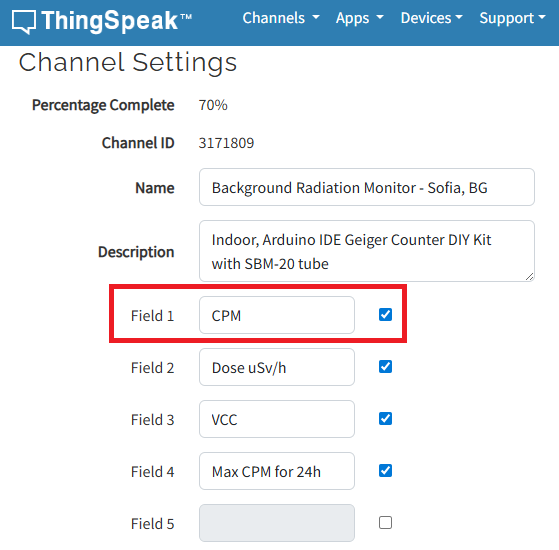
I have to say that I'm not an engineer or coder, just can simply load some Arduino sketches and few more things, so I'll be very thankfull if someone could explain like for non-IT users.
Regards,
Emo
Experimenting with Agentic AI
44%
I am an AI skeptic
0%
AI is banned at work
11%
I am happy with Conversational AI
44%
9 votes

It’s exciting to dive into a new dataset full of unfamiliar variables but it can also be overwhelming if you’re not sure where to start. Recently, I discovered some new interactive features in MATLAB live scripts that make it much easier to get an overview of your data. With just a few clicks, you can display sparklines and summary statistics using table variables, sort and filter variables, and even have MATLAB generate the corresponding code for reproducibility.
The Graphics and App Building blog published an article that walks through these features showing how to explore, clean, and analyze data—all without writing any code.
If you’re interested in streamlining your exploratory data analysis or want to see what’s new in live scripts, you might find it helpful:
If you’ve tried these features or have your own tips for quick data exploration in MATLAB, I’d love to hear your thoughts!
Pure Matlab
82%
Simulink
18%
11 votes
Jorge Bernal-AlvizJorge Bernal-Alviz shared the following code that requires R2025a or later:
Test()

function Test()
duration = 10;
numFrames = 800;
frameInterval = duration / numFrames;
w = 400;
t = 0;
i_vals = 1:10000;
x_vals = i_vals;
y_vals = i_vals / 235;
r = linspace(0, 1, 300)';
g = linspace(0, 0.1, 300)';
b = linspace(1, 0, 300)';
r = r * 0.8 + 0.1;
g = g * 0.6 + 0.1;
b = b * 0.9 + 0.1;
customColormap = [r, g, b];
figure('Position', [100, 100, w, w], 'Color', [0, 0, 0]);
axis equal;
axis off;
xlim([0, w]);
ylim([0, w]);
hold on;
colormap default;
colormap(customColormap);
plothandle = scatter([], [], 1, 'filled', 'MarkerFaceAlpha', 0.12);
for i = 1:numFrames
t = t + pi/240;
k = (4 + 3 * sin(y_vals * 2 - t)) .* cos(x_vals / 29);
e = y_vals / 8 - 13;
d = sqrt(k.^2 + e.^2);
c = d - t;
q = 3 * sin(2 * k) + 0.3 ./ (k + 1e-10) + ...
sin(y_vals / 25) .* k .* (9 + 4 * sin(9 * e - 3 * d + 2 * t));
points_x = q + 30 * cos(c) + 200;
points_y = q .* sin(c) + 39 * d - 220;
points_y = w - points_y;
CData = (1 + sin(0.1 * (d - t))) / 3;
CData = max(0, min(1, CData));
set(plothandle, 'XData', points_x, 'YData', points_y, 'CData', CData);
brightness = 0.5 + 0.3 * sin(t * 0.2);
set(plothandle, 'MarkerFaceAlpha', brightness);
drawnow;
pause(frameInterval);
end
end
From my experience, MATLAB's Deep Learning Toolbox is quite user-friendly, but it still falls short of libraries like PyTorch in many respects. Most users tend to choose PyTorch because of its flexibility, efficiency, and rich support for many mathematical operators. In recent years, the number of dlarray-compatible mathematical functions added to the toolbox has been very limited, which makes it difficult to experiment with many custom networks. For example, svd is currently not supported for dlarray inputs.
This link (List of Functions with dlarray Support - MATLAB & Simulink) lists all functions that support dlarray as of R2026a — only around 200 functions (including toolbox-specific ones). I would like to see support for many more fundamental mathematical functions so that users have greater freedom when building and researching custom models. For context, the core MATLAB mathematics module contains roughly 600 functions, and many application domains build on that foundation.
I hope MathWorks will prioritize and accelerate expanding dlarray support for basic math functions. Doing so would significantly increase the Deep Learning Toolbox's utility and appeal for researchers and practitioners.
Thank you.
Run MATLAB using AI applications by leveraging MCP. This MCP server for MATLAB supports a wide range of coding agents like Claude Code and Visual Studio Code.
Check it out and share your experiences below. Have fun!
GitHub repo: https://github.com/matlab/matlab-mcp-core-server
Yann Debray's blog post: https://blogs.mathworks.com/deep-learning/2025/11/03/releasing-the-matlab-mcp-core-server-on-github/
как я получил api Token
I just learned you can access MATLAB Online from the following shortcut in your web browser: https://matlab.new
Thanks @Yann Debray
From his recent blog post: pip & uv in MATLAB Online » Artificial Intelligence - MATLAB & Simulink