Results for
Web Automation with Claude, MATLAB, Chromium, and Playwright
Duncan Carlsmith, University of Wisconsin-Madison
Introduction
Recent agentic browsers (Chrome with Claude Chrome extension and Comet by Perplexity) are marvelous but limited. This post describes two things: first, a personal agentic browser system that outperforms commercial AI browsers for complex tasks; and second, how to turn AI-discovered web workflows into free, deterministic MATLAB scripts that run without AI.
My setup is a MacBook Pro with the Claude Desktop app, MATLAB 2025b, and Chromium open-source browser. Relevant MCP servers include fetch, filesystem, MATLAB, and Playwright, with shell access via MATLAB or shell MCP. Rather than use my Desktop Chrome application, which might expose personal information, I use an independent, dedicated Chromium with a persistent login and preauthentication for protected websites. Rather than screenshots, which quickly saturate a chat context and are expensive, I use the Playwright MCP server, which accesses the browser DOM and accessibility tree directly. DOM manipulation permits error-free operation of complex web page UIs.
The toolchain required is straightforward. You need Node.js , which is the JavaScript runtime that executes Playwright scripts outside a browser. Install it, then set up a working directory and install Playwright with its bundled Chromium:
# Install Node.js via Homebrew (macOS) or download from nodejs.org
brew install node
# Create a working directory and install Playwright
mkdir MATLABWithPlaywright && cd MATLABWithPlaywright
npm init -y
npm install playwright
# Download Playwright's bundled Chromium (required for Tier 1)
npx playwright install chromium
That is sufficient for the Tier 1 examples. For Tier 2 (authenticated automation), you also need Google Chrome or the open-source Chromium browser, launched with remote debugging enabled as described below. Playwright itself is an open-source browser automation library from Microsoft that can either launch its own bundled browser or connect to an existing one -- this dual capability is the foundation of the two-tier architecture. For the AI-agentic work described in the Canvas section, you need Claude Desktop with MCP servers configured for filesystem access, MATLAB, and Playwright. The INSTALL.md in the accompanying FEX submission covers all of this in detail.
AI Browser on Steroids: Building Canvas Quizzes
An agentic browser example just completed illustrates the power of this approach. I am adding a computational thread to a Canvas LMS course in modern physics based on relevant interactive Live Scripts I have posted to the MATLAB File Exchange. For each of about 40 such Live Scripts, I wanted to build a Canvas quiz containing an introduction followed by a few multiple-choice questions and a few file-upload questions based on the "Try this" interactive suggestions (typically slider parameter adjustments) and "Challenges" (typically to extend the code to achieve some goal). The Canvas interface for quiz building is quite complex, especially since I use a lot of LaTeX, which in the LMS is rendered using MathJax with accessibility features and only a certain flavor of encoding works such that the math is rendered both in the quiz editor and when the quiz is displayed to a student.
My first prompt was essentially "Find all of my FEX submissions and categorize those relevant to modern physics.” The categories emerged as Relativity, Quantum Mechanics, Atomic Physics, and Astronomy and Astrophysics. Having preauthenticated at MathWorks with a Shibboleth university license authentication system, the next prompt was "Download and unzip the first submission in the relativity category, read the PDF of the executed script or view it under examples at FEX, then create quiz questions and answers as described above." The final prompt was essentially "Create a new quiz in my Canvas course in the Computation category with a due date at the end of the semester. Include the image and introduction from the FEX splash page and a link to FEX in the quiz instructions. Add the MC quiz questions with 4 answers each to select from, and the file upload questions. Record what you learned in a SKILL file in my MATLAB/claude/SKILLS folder on my filesystem." Claude offered a few options, and we chose to write and upload the quiz HTML from scratch via the Canvas REST API. Done. Finally, "Repeat for the other FEX File submissions." Each took a couple of minutes. The hard part was figuring out what I wanted to do exactly.
Mind you, I had tried to build a Canvas quiz including LaTeX and failed miserably with both Chrome Extension and Comet. The UI manipulations, especially to handle the LaTeX, were too complex, and often these agentic browsers would click in the wrong place, wind up on a different page, even in another tab, and potentially become destructive.
A key gotcha with LaTeX in Canvas: the equation rendering system uses double URL encoding for LaTeX expressions embedded as image tags pointing to the Canvas equation server. The LaTeX strings must use single backslashes -- double backslashes produce broken output. And Canvas Classic Quizzes and New Quizzes handle MathJax differently, so you need to know which flavor your institution uses.
From AI-Assisted to Programmatic: The Two-Tier Architecture
An agentic-AI process, like the quiz creation, can become expensive. There is a lot of context, both physics content-related and process-related, and the token load mounts up in a chat. Wouldn't it be great if, after having used the AI for what it is best at -- summarizing material, designing student exercises, and discovering a web-automation process -- one could repeat the web-related steps programmatically for free with MATLAB? Indeed, it would, and is.
In my setup, usually an AI uses MATLAB MCP to operate MATLAB as a tool to assist with, say, launching an application like Chromium or to preprocess an image. But MATLAB can also launch any browser and operate it via Playwright. (To my knowledge, MATLAB can use its own browser to view a URL but not to manipulate it.) So the following workflow emerges:
1) Use an AI, perhaps by recording the DOM steps in a manual (human) manipulation, to discover a web-automation process.
2) Use the AI to write and debug MATLAB code to perform the process repeatedly, automatically, for free.
I call this "temperature zero" automation -- the AI contributes entropy during workflow discovery, then the deterministic script is the ground state.
The architecture has three layers:
MATLAB function (.m)
|
v
Generate JavaScript/Playwright code
|
v
Write to temporary .js file
|
v
Execute: system('node script.js')
|
v
Parse output (JSON file or console)
|
v
Return structured result to MATLAB
The .js files serve double duty: they are both the runtime artifacts that MATLAB generates and executes, AND readable documentation of the exact DOM interactions Playwright performs. Someone who wants to adapt this for their own workflow can read the .js file and see every getByRole, fill, press, and click in sequence.
Tier 1: Basic Web Automation Examples
I have demonstrated this concept with three basic examples, each consisting of a MATLAB function (.m) that dynamically generates and executes a Playwright script (.js). These use Playwright's bundled Chromium in headless mode -- no authentication required, no persistent sessions.
01_ExtractTableData
extractTableData.m takes a URL and scrapes a complex Wikipedia table (List of Nearest Stars) that MATLAB's built-in webread cannot handle because the table is rendered by JavaScript. The function generates extract_table.js, which launches Playwright's bundled Chromium headlessly, waits for the full DOM to render, walks through the table rows extracting cell text, and writes the result as JSON. Back in MATLAB, the JSON is parsed and cleaned (stripping HTML tags, citation brackets, and Unicode symbols) into a standard MATLAB table.
T = extractTableData(...
'https://en.wikipedia.org/wiki/List_of_nearest_stars_and_brown_dwarfs');
disp(T(1:5, {'Star_name', 'Distance_ly_', 'Stellar_class'}))
histogram(str2double(T.Distance_ly_), 20)
xlabel('Distance (ly)'); ylabel('Count'); title('Nearest Stars')
02_ScreenshotWebpage
screenshotWebpage.m captures screenshots at configurable viewport dimensions (desktop, tablet, mobile) with full-page or viewport-only options. The physics-relevant example captures the NASA Webb Telescope page at multiple viewport sizes. This is genuinely useful for checking how your own FEX submission pages or course sites look on different devices.
03_DownloadFile
downloadFile.m is the most complex Tier 1 function because it handles two fundamentally different download mechanisms. Direct-link downloads (where navigating to the URL triggers the download immediately) throw a "Download is starting" error that is actually success:
try {
await page.goto(url, { waitUntil: 'commit' });
} catch (e) {
// Ignore "Download is starting" -- that means it WORKED!
if (!e.message.includes('Download is starting')) throw e;
}
Button-click downloads (like File Exchange) require finding and clicking a download button after page load. The critical gotcha: the download event listener must be set up BEFORE navigation, not after. Getting this ordering wrong was one of those roadblocks that cost real debugging time.
The function also supports a WaitForLogin option that pauses automation for 45 seconds to allow manual authentication -- a bridge to Tier 2's persistent-session approach.
Another lesson learned: don't use Playwright for direct CSV or JSON URLs. MATLAB's built-in websave is simpler and faster for those. Reserve Playwright for files that require JavaScript rendering, button clicks, or authentication.
Tier 2: Production Automation with Persistent Sessions
Tier 2 represents the key innovation -- the transition from "AI does the work" to "AI writes the code, MATLAB does the work." The critical architectural difference from Tier 1 is a single line of JavaScript:
// Tier 1: Fresh anonymous browser
const browser = await chromium.launch();
// Tier 2: Connect to YOUR running, authenticated Chrome
const browser = await chromium.connectOverCDP('http://localhost:9222');
CDP is the Chrome DevTools Protocol -- the same WebSocket-based interface that Chrome's built-in developer tools use internally. When you launch Chrome with a debugging port open, any external program can connect over CDP to navigate pages, inspect and manipulate the DOM, execute JavaScript, and intercept network traffic. The reason this matters is that Playwright connects to your already-running, already-authenticated Chrome session rather than launching a fresh anonymous browser. Your cookies, login sessions, and saved credentials are all available. You launch Chrome once with remote debugging enabled:
/Applications/Google\ Chrome.app/Contents/MacOS/Google\ Chrome \
--remote-debugging-port=9222 \
--user-data-dir="$HOME/chrome-automation-profile"
Log into whatever sites you need. Those sessions persist across automation runs.
addFEXTagLive.m
This is the workhorse function. It uses MATLAB's modern arguments block for input validation and does the following: (1) verifies the CDP connection to Chrome is alive with a curl check, (2) dynamically generates a complete Playwright script with embedded conditional logic -- check if tag already exists (skip if so), otherwise click "New Version", add the tag, increment the version number, add update notes, click Publish, confirm the license dialog, and verify the success message, (3) executes the script asynchronously and polls for a result JSON file, and (4) returns a structured result with action taken, version changes, and optional before/after screenshots.
result = addFEXTagLive( ...
'https://www.mathworks.com/matlabcentral/fileexchange/183228-...', ...
'interactive_examples', Screenshots=true);
% result.action is either 'skipped' or 'added_tag'
% result.oldVersion / result.newVersion show version bump
% result.screenshots.beforeImage / afterImage for display
The corresponding add_fex_tag_production.js is a standalone Node.js version that accepts command-line arguments:
node add_fex_tag_production.js 182704 interactive-script 0.01 "Added tag"
This is useful for readers who want to see the pure JavaScript logic without the MATLAB generation layer.
batch_tag_FEX_files.m
The batch controller reads a text file of URLs, loops through them calling addFEXTagLive with rate limiting (10 seconds between submissions), tracks success/skip/fail counts, and writes three output files: successful_submissions.txt, skipped_submissions.txt, and failed_submissions_to_retry.txt.
This script processed all 178 of my FEX submissions:
Total: 178 submissions processed in 2h 11m (~44 sec/submission)
Tags added: 146 (82%) | Already tagged: 32 (18%) | True failures: 0
Manual equivalent: ~7.5 hours | Token cost after initial engineering: $0
The Timeout Gotcha
An interesting gotcha emerged during the batch run. Nine submissions were reported as failures with timeout errors. The error message read:
page.textContent: Timeout 30000ms exceeded.
Call log: - waiting for locator('body')
Investigation revealed these were false negatives. The timeout occurred in the verification phase -- Playwright had successfully added the tag and clicked Publish, but the MathWorks server was slow to reload the confirmation page (>30 seconds). The tag was already saved. When a retry script ran, all nine immediately reported "Tag already exists -- SKIPPING." True success rate: 100%.
Could this have been fixed with a longer timeout or a different verification strategy? Sure. But I mention it because in a long batch process (2+ hours, 178 submissions), gotchas emerge intermittently that you never see in testing on five items. The verification-timeout pattern is a good one to watch for: your automation succeeded, but your success check failed.
Key Gotchas and Lessons Learned
A few more roadblocks worth flagging for anyone attempting this:
waitUntil options matter. Playwright's networkidle wait strategy almost never works on modern sites because analytics scripts keep firing. Use load or domcontentloaded instead. For direct downloads, use commit.
Quote escaping in MATLAB-generated JavaScript. When MATLAB's sprintf generates JavaScript containing CSS selectors with double quotes, things break. Using backticks as JavaScript template literal delimiters avoids the conflict.
The FEX license confirmation popup is accessible to Playwright as a standard DOM dialog, not a browser popup. No special handling needed, but the Publish button appears twice -- once to initiate and once to confirm -- requiring exact: true in the role selector to distinguish them:
// First Publish (has a space/icon prefix)
await page.getByRole('button', { name: ' Publish' }).click();
// Confirm Publish (exact match)
await page.getByRole('button', { name: 'Publish', exact: true }).click();
File creation from Claude's container vs. your filesystem. This caused real confusion early on. Claude's default file creation tools write to a container that MATLAB cannot see. Files must be created using MATLAB's own file operations (fopen/fprintf/fclose) or the filesystem MCP's write_file tool to land on your actual disk.
Selector strategy. Prefer getByRole (accessibility-based, most stable) over CSS selectors or XPath. The accessibility tree is what Playwright MCP uses natively, and role-based selectors survive minor UI changes that would break CSS paths.
Two Modes of Working
Looking back, the Canvas quiz creation and the FEX batch tagging represent two complementary modes of working with this architecture:
The Canvas work keeps AI in the loop because each quiz requires different physics content -- the AI reads the Live Script, understands the physics, designs questions, and crafts LaTeX. The web automation (posting to Canvas via its REST API) is incidental. This is AI-in-the-loop for content-dependent work.
The FEX tagging removes AI from the loop because the task is structurally identical across 178 submissions -- navigate, check, conditionally update, publish. The AI contributed once to discover and encode the workflow. This is AI-out-of-the-loop for repetitive structural work.
Both use the same underlying architecture: MATLAB + Playwright + Chromium + CDP. The difference is whether the AI is generating fresh content or executing a frozen script.
Reference Files and FEX Submission
All of the Tier 1 and Tier 2 MATLAB functions, JavaScript templates, example scripts, installation guide, and skill documentation described in this post are available as a File Exchange submission: Web Automation with Claude, MATLAB, Chromium, and Playwright .The package includes:
Tier 1 -- Basic Examples:
- extractTableData.m + extract_table.js -- Web table scraping
- screenshotWebpage.m + screenshot_script.js -- Webpage screenshots
- downloadFile.m -- File downloads (direct and button-click)
- Example usage scripts for each
Tier 2 -- Production Automation:
- addFEXTagLive.m -- Conditional FEX tag management
- batch_tag_FEX_files.m -- Batch processing controller
- add_fex_tag_production.js -- Standalone Node.js automation script
- test_cdp_connection.js -- CDP connection verification
Documentation and Skills:
- INSTALL.md -- Complete installation guide (Node.js, Playwright, Chromium, CDP)
- README.md -- Package overview and quick start
- SKILL.md -- Best practices, decision trees, and troubleshooting (developed iteratively through the work described here)
The SKILL.md file deserves particular mention. It captures the accumulated knowledge from building and debugging this system -- selector strategies, download handling patterns, wait strategies, error handling templates, and the critical distinction between when to use Playwright versus MATLAB's native websave. It was developed as a "memory" for the AI assistant across chat sessions, but it serves equally well as a human-readable reference.
Credits and conclusion
This synthesis of existing tools was conceived by the author, but architected (if I may borrow this jargon) by Claud.ai. This article was conceived and architected by the author, but Claude filled in the details, most of which, as a carbon-based life form, I could never remember. The author has no financial interest in MathWorks or Anthropic.
Anthropic has just announced Claude’s Constitution to govern Claude’s behavior in anticipation of a continued ramp-up to AGI abilities. Amusing me just now, just as this constitution was announced, I was encountering a wee moral dilemma myself with Claude.
Claude and I were trying to transfer all of Claude’s abilities and knowledge for controlling macOS and iPhone apps in my setup (See A universal agentic AI for your laptop and beyond) to the Perplexity App. My macOS Perplexity App is configured with the full suite of MCP services available to my Claude App, but I hadn’t yet exercised these with Perplexity App. Oddly, all but Playwright failed to work despite our many experiments and searches for information at Perplexity and elsewhere.
I suspect that Perplexity built into the macOS app all the hooks for MCP, but became gun-shy for security reasons and enforced constraints so none of its models (not even the very model Claude App was running) can execute MCP-related commands, oddly except those for PlayWright. The Perplexity App even offers a few of its own MCP connectors, but these are also non-functional. It is possible we missed something. These limitations appear to be undocumented.
Pulling our hair out, Claude and I were wondering how such constraints might be implemented, and Claude suggested an experiment and then a possible workaround. At that point, I had to pause and say, “No, we are not going there.” No, I won’t tell you the suggested workaround. No, we didn’t try it. Tempting in the moment, but no.
Be safe. And be a good person. Don’t let your enthusiasm reign unbridled.
Disclosure: The author has no direct financial interest in Anthropic, and loves Perplexity App and Comet too, but his son (a philosopher by training) is the lead author on this draft of the Constitution, and overuses the phrase “broadly speaking” in my opinion.
This article describes how to prototype a physics simulation in HTML5 with Claude desktop App and then to replicate and deploy this product in MATLAB as an interactive GUI script. It also demonstrates how to use Claude Chrome Extension to operate MATLAB Online and App Designer to build bonafide MATLAB Apps with AI online.
Setup
My setup is a MacBook with Claude App with MATLAB (v2025a), MATLAB MCP Core Serve,r and various cloud related MCP tools. This setup allows Claude App to operate MATLAB locally and to manage files. I also have Claude Chrome Extension. A new feature in Claude App is a coding tab connected to Claude code file management locally.
Building HTML5 and MATLAB interactive applications with Claude App
In exploring the new Claude App tab, Claude suggested a variety of projects and I elected to build an HTML5 physics simulation. The Claude App interface has built-in rendering for artifacts including .html, .jsx, .svg, .md, .mermaid, and .pdf so an HTML5 interactive app artifact produced appears active right in Claude App. That’s fun and I had the thought that HTML5 would be a speedy way to prototype MATLAB code without evenconnecting to MATLAB.
I chose to simulateof a double pendulum, well known to exhibit chaotic motion, a simulation that students and instructors of physics might use to easily explore chaos interactively. I knew the project would entail numerical integration so was not entirely trivial in HTML5, and would later be relatively easy and more precise in MATLAB using ode45.
One thing led to another and shortly I had built a prototype HTML5 interactive app and then a MATLAB version and deployed it to my MATLAB Apps library. I didn’t write a line of code. Everything I describe and exhibit here was AI generated. It could have been hands-free. I can talk to Claude via Siri or via an interface Claude helped me build using MATLAB speech-to-text ( I have taught Claude to speak its responses back to me but that’s another story.)
A remarkable thing I learned is not just the AI’s ability to write HTML5 code in addition to MATLAB code, but its knowledge and intuition about app layout and user interactions. I played the role of an increasingly demanding user-experience tester, exercising and providing feedback on the interface, issuing prompts like “Add drag please” (Voila, a new drag slider with appropriately set limits and default value appears.) and “I want to be able to drag the pendulum masses, not just set angles via sliders, thank you.” Then “Convert this into a MATLAB code.”
I was essentially done in 45 minutes start to finish, added a last request, and went to bed. This morning I was just wondering and asked, “Any chance we can make this a MATLAB App?” and voila it was packaged and added to my Apps Library with an install file for others to use it. I will park these products on File Exchange for those who want to try out the Double Pendulum simulation. Later I realized this was not exactly what I had in mind
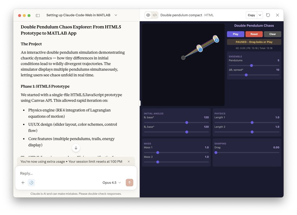
The screenshot below shows the Claude interface at the end of the process. The HTML5 product is fully operational in the artifacts pane on the right. One can select the number of simultaneous pendulums and ranges for initial conditions and click the play button right there in Claude App to observe how small perturbations result in divergence in the motions (chaos) for large pendulum angles, and the effect of damping.
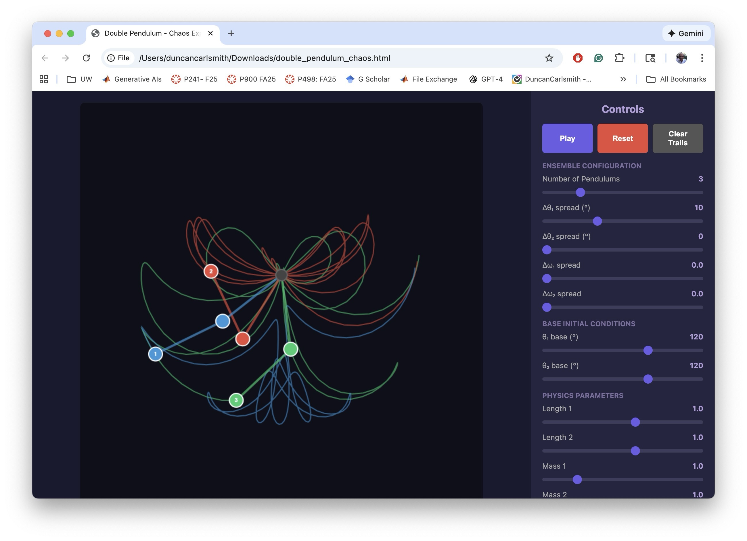
The following image below show the HTML5 in a Chrome Browser window.
I making the MATLAB equivalent of the HTML5 app, I iterated a bit on the interactive features. The app has to trap user actions, consider possible sequences of choices, and be aware of timing. Success and satisfaction took several iteractions.
The screenshot below shows the final interactive MATLAB .m script running in MATLAB. The script creates a figure with interactive controls mirroring the HTML5 version. The DoublePendulumApp.mlappinstall file in the Files pane, created by Claude, copies the .m to the MATLAB/Apps folder and adds a button to the APPS Tab in the MATLAB tool strip.

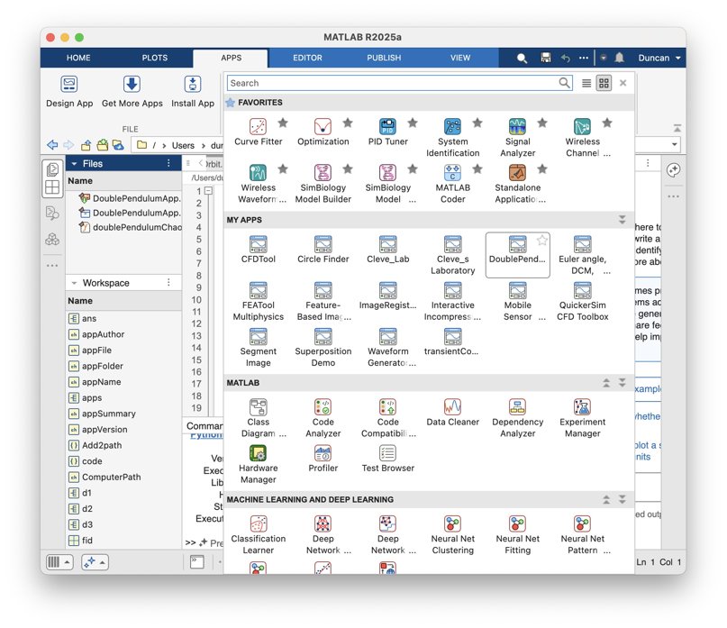
Below, you can see the MATLAB APP in my Apps Library.
To be clear, what was created in this process was not a true .mlapp binary file that would be created by MATLAB App Designer. In my setup, with MATLAB operating locally, Claude has no access to App Designer interactive windows via Puppeteer. It might be given access via some APPLE Script or other OS-specific trick but I’ve not pursued such options.
Claude Chrome Extension and App Designer online
To test if one could build actual Apps in the MATLAB sense with App Designer and Claude, I opened Claude Chrome Extension (beta) in Chrome in one tab and logged into MATLAB Online in another. Via the Chrome extension, Claude has access to the MATLAB Online IDE GUI and command line. I asked Claude to open App Designer and make a start on a prototype project. It can ferreted around in available MathWorks documentation, used MATLAB Online help vi the GUI I think, and performed some experiments to understand how to operate App Designer, and figured it out.
The screenshot below demonstrates a succesful first test of building an App Designer app from scratch. On the left is part of a Chrome window showing the Claude AI interface on the right hand side of a Chrome tab that is mostly off screen. On the right in the screenshot is MATLAB App Designer in a Chrome tab. A first button has been dragged on to the Design View frame in App Designer.

I only wanted to know if this workflow was possible, not build say the random quote generator Claude suggested. I have successfully operated MATLAB Online via Perplexity Comet Browser but not tried to operate APP Designer. Comet might be an alternate choice for this sort of task.
A word of caution. It is not clear to me that a Chrome Extension chat is available post facto through your regular Claude account, yet.
Appendix
This appendix is a summary generated by Claude of the development process and offers some additional details.
Double Pendulum Chaos Explorer: From HTML5 Prototype to MATLAB App
Author: Claude (Anthropic)
The Project
An interactive double pendulum simulation demonstrating chaotic dynamics — how tiny differences in initial conditions lead to wildly divergent trajectories. The simulator displays multiple pendulums simultaneously, letting users see chaos unfold in real time.
Phase 1: HTML5 Prototype
We started with a single-file HTML5/JavaScript prototype using Canvas API. This allowed rapid iteration on:
• Physics engine (RK4 integration of Lagrangian equations of motion)
• UI/UX design (slider layout, color schemes, control flow)
• Core features (multiple pendulums, trails, energy display)
The HTML5 version served as a "living specification" — we could test ideas in the browser instantly before committing to MATLAB implementation.
Phase 2: MATLAB GUI Development
Converting to MATLAB revealed platform-specific challenges:
Function name conflicts — Internal function names like updateFrame collided with Robotics Toolbox. Solution: prefix all functions with dp (e.g., dpUpdateFrame).
Timer-based animation — MATLAB's timer callbacks require careful state management via fig.UserData.
Robustness — Users can interact with sliders mid-animation. Every callback needed try-catch protection and proper pause/reinitialize logic.
Graphics cleanup — Changing pendulum count mid-run left orphaned graphics objects. Fixed with explicit cla() and handle deletion.
Key insight: The HTML5 prototype's logic translated almost directly, but MATLAB's callback architecture demanded defensive programming throughout.
Phase 3: MATLAB App Packaging
The final .m file was packaged as an installable MATLAB App using matlab.apputil.package(). This creates a .mlappinstall file that:
• Installs with a double-click
• Appears in MATLAB's APPS toolbar
• Can be shared with colleagues who have MATLAB
Files Produced
double_pendulum_chaos.html — Standalone browser version
doublePendulumChaosExplorer.m — MATLAB source code
DoublePendulumApp.mlappinstall — Shareable MATLAB App installer
Takeaways
1. Prototype in HTML5 — Fast iteration, instant feedback, platform-independent testing
2. Port to MATLAB — Same physics, different UI paradigm; expect callback/state management work
3. Package as App — One command turns a .m file into a distributable app
The whole process — from first HTML5 sketch to installed MATLAB App — demonstrates how rapid prototyping in the browser can accelerate development of production tools in specialized environments like MATLAB.
Introduction
This article describes how I have used MATLAB, MCP, and other tools to enable AI desktop apps to communicate with and share information between multiple AIs in performing research and code development. I describe how Claude desktop app (for example) can orchestrate AI-related setups of itself and other AI dektop apps using system calls through MATLAB, access multiple local and cloud AIs to develop and test code, and share with and evaluate results from multiple AIs. If you have been copy-pasting between MATLAB and an AI application or browser page, you may find this helpful.
Warning
When connected to MATLAB App via MCP, an AI desktop application acquires MATLAB App's command line privileges, possibly full system privileges. Be careful what commands you approve.
Setup
Experiments with Claude code and MATLAB MCP Core Server describes how to link Claude App via MCP to a local MATLAB to create MATLAB scripts in your file system, operate MATLAB App to test them, collect errors sent to standard output, view created files, and iterate. Other AI apps can similarly configured as described here.
My setup is an APPLE M1 MacBook with MATLAB v2025a and ollama along with MATLAB MCP Core Server, ollama MCP, filesystem MCP, fetch MCP to access web pages, and puppeteer MCP to navigate and operate webpages like MATLAB Online. I have similarly Claude App, Perplexity App (which requires the PerplexityXPC helper for MCP since it's sandboxed as a Mac App Store app), and LM Studio App. As of this writing, ChatGPT App support for MCP connectors is currently in beta and possibly available to Pro users if setup enabled via a web browser. It is not described here.
The available MCP commands are:
filesystem MCP `read_text_file`, `read_media_file`, `write_file`, `edit_file`, `list_directory`, `search_files`, `get_file_info`, etc.
matlab MCP `evaluate_matlab_code`, `run_matlab_file`, `run_matlab_test_file`, `check_matlab_code`, `detect_matlab_toolboxes`
fetch MCP ‘fetch_html`, `fetch_markdown`, `fetch_txt`, `fetch_json` | Your Mac |
puppeteer MCP `puppeteer_navigate`, `puppeteer_screenshot`, `puppeteer_click`, `puppeteer_fill`, `puppeteer_evaluate`, etc.
ollama MCP ‘ollama_list’, ‘ollama_show’, ’ollama_pull’, ’ollama_push’, ’ollana_copy’, ’ ollama-create’, ’ollama_copy’, ’ollama_delete’, ’ollama_ps’, ’ollama_chat’, ’ollama_web_search’, ’ollama_web_fetch’
Claude App (for example) can help you find, download, install, and configure MCP services for itself and for other Apps. Claude App requires for this setup a json configuration file like
{
"mcpServers": {
"ollama": {
"command": "npx",
"args": ["-y", "ollama-mcp"],
"env": {
"OLLAMA_HOST": "http://localhost:11434"
}
},
"filesystem": {
"command": "npx",
"args": [
"-y",
"@modelcontextprotocol/server-filesystem",
"/Users/duncancarlsmith/Documents/MATLAB"
]
},
"matlab": {
"command": "/Users/duncancarlsmith/Developer/mcp-servers/matlab-mcp-core-server",
"args": ["--matlab-root", "/Applications/MATLAB_R2025a.app"]
},
"fetch": {
"command": "npx",
"args": ["-y", "mcp-fetch-server"]
},
"puppeteer": {
"command": "npx",
"args": ["-y", "@modelcontextprotocol/server-puppeteer"]
}
}
}
Various options for these services are available through Claude App’s Settings=>Connectors. If you first install and set up the MATLAB MCP with Claude App, then Claude can find and edit its own json file using MATLAB and help you (after quitting and restarting) to complete the installations of all of the other tools. I highly recommend using Claude App as a command post for installations although other desktop apps like Perplexity may serve equally well.
Perplexity App is manually configured using Settings=>Connectors and adding server names and commands as above. Perplexity XPC is included with the Perplexity App download . When you create connectors with Perplexity App, you are prompted to install Perplexity XPC to allow Perplexity App to spawn proceses outside its container. LM Studio is manually configured via its righthand sidebar terminal icon by selecting Install-> Edit mcp.json. The json is like Claude’s. Claude can tell/remind you exactly what to insert there.
One gotcha in this setup concerns the Ollama MCP server. Apparently the default json format setting fails and one must tell the AIs to use “markdown” when commuicating with it. This instruction can be made session by session but I have made it a permanent preference in Claude App by clicking my initials in the lower left of Claude App, selecting settings, and under “What preferences should claude consider in responses,” adding “When using ollama MCP tools (ollama_chat, ollama_generate), always set format="markdown" - the default json format returns empty responses.”
LM Studio by default points at an Open.ai API. Claude can tell you how to download a model, point LM Studio at a local Ollama model and set up LM Studio App with MCP. Be aware that the default context setting in LM Studio is too small. Be sure to max out the context slider for your selected model or you will experience an AI with a very short term memory and context overload failures. When running MATLAB, LM Studio will ask for a project directory. Under presets you can enter something like “When using MATLAB tools, always use /Users/duncancarlsmith/Documents/MATLAB as the project_path unless the user specifies otherwise.” and attach that to the context in any new chat. An alternate ollama desktop application is Ollama from ollama.com which can run large models in the cloud. I encountered some constraints with Ollama App so focus on LM Studio.
I have installed Large Language Models (LLMs) with MATLAB using the recommended Add-on Browser. I had Claude configure and test it. This package helps MATLAB communicate with external AIs via API and also with my native ollama. See the package information. To use it, one must define tools with MATLAB code. A tool is a function with a description that tells an LLM what the function does, what parameters it takes, and when to call it. FYI, Claude discovered my small ollama default model had not been trained to support tool and hallucinated a numerical calculaton rather than using a tool we set up to perform such a calculation with MATLAB with machine precision. Claude suggested and then orchestrated the download of the 7.1 GB model mistral-nemo model which supports tool calling so if using you are going to use tools be sure to use a tool aware model.
To interact with Ollama, Claude can use the MATLAB MCP server to execute MATLAB commands to use ollamaChat() from the LLMs-with-MATLAB package like “chat = ollamaChat("mistral-nemo");response = generate(chat, "Your question here”);” The ollamaChat function creates an object that communicates with Ollama's HTTP API running on localhost:11434. The generate function sends the prompt and returns the text response. Claude can also communicate with Ollama using the Ollama MCP server. Similarly, one can ask Claude to create tools for other AIs.
The tool capability allows one to define and suggest MATLAB functions that the Ollama model can request to use to, for example, to make exact numerical calculations in guiding its response. I have also the MATLAB Add-on MATLAB MCP HTTP Client which allows MATLAB to connect with cloud MCP servers. With this I can, for example, connect to an external MCP service to get JPL-quality (SPICE generated) ephemeris predictions for solar system objects and, say, plot Earth’s location in solar system barycentric coordinates and observe the deviations from a Keplerian orbit due of lunar and other gravitational interactions.
To connect with an external AI API such as openAI or Perplexity, you need an account and API key and this key must be set as an environmental variable in MATLAB. Claude can remind you how to create the environmental variable by hand or how you can place your key in a file and have Claude find and extract the key and define the environmental variable without you supplying it explicitly to Claude.
It should be pointed out that conversations and information are NOT shared between Desktop apps. For example, if I use Claude App to, via MATLAB, make an API transaction with ChatGPT or Perplexity in the cloud, the corresponding ChatGPT App or Perplexity App has no access the the transaction, not even to a log file indicating it occured. There may be various OS dependent tricks to enable communication between AI desktop apps (e.g. AppleScript/AppleEvents copy and paste) but I have not explored such options.
AI<->MATLAB Communication
WIth this setup, I can use any of the three desktop AI apps to create and execute a MATLAB script or to ask any supported LLM to do this. Only runtime standard output text like error messages generated by MATLAB are fed back via MCP. Too evaluate the results of a script during debugging and after successful execution, an AI requires more information.
Perplexity App can “see and understand” binary graphical output files (presented as inputs to the models like other data) without human intervention via screen sharing, obviating the need to save or paste figures. Perplexity and Claude can both “see” graphical output files dragged and dropped manually into their prompt interface. With MacOS, I can use Shift-Command-5 to capture a window or screen selection and paste it into the input field in either App. Can this exchange of information be accomplished programmatically? Yes, using MCP file services.
To test what binary image file formats are supported by Claude with the file server connection, I asked Claude to use MATLAB commands to make and convert a figure to JPEG, PNG, GIF, BMP, TIFF, and WebP and found the filesytem: read_media_file command of the Claude file server connection supported the first three. The file server MCP transmits the file using JSON and base64 text strings. A 64-bit encoding adds an additonal ~30 percent to a bitmap format and there is overhead. A total tranmission limit of 1MB is imposed by Anthropic so the maximum bitmap file size appears to be about 500 KB. If your output graphic file is larger, you may ask Claude to use MATLAB to compress it before reading it via the file service.
BTW, interestingly, the drag and drop method of image file transfer does not have this 500 KB limit. I dragged and dropped an out of context (never shared in my interactions with Claude) 3.3 MB JPEG and received a glowing, detailed description of my cat.
So in in generating a MATLAB script via AI prompts, we can ask the AI to make sure MATLAB commands are included in the script that save every figure in a supported and possibly compressed bitmap format so the command post can fetch it. Claude, for example, can ‘see’ an an annotated plot and and accurately describe the axes labels, understand the legend, extract numbers in an annotation, and also derive approximate XY values of a plotted function. Note that Claude (given some tutoring and an example) can also learn to parse and find all of the figures saved as PNG inside a saved .mlx package and, BTW, create a .mlx from scratch. So an alternate path is to generate a Live Script or ask the AI to convert a .m script to Live Script using a MATLAB command and to save the executed .mlx. Another option is for the AI to ask MATLAB to loop over figures and execute for each issue a command like exportgraphics(fig, ‘figname.png', 'Resolution', 150); and then itself upload the files for processing.
With a sacrifiice of security, other options are available. With the APPLE OS, it is possible to approve matlab_mcp_core_server (and or your Claude App or Perplexity App) to access screen and audio recording. Then for example, Claude can ask MATLAB to issue a system command system('screencapture -x file.png') to capture the entire screen or java.awt.Robot().createScreenCapture() to capture a screen window. I have demonstrated with Claude App capturing a screenshot showing MATLAB App and figures, and, for fun, sending that via API to ChatGPT, and receiving back an analysis of the contents. (Sending the screenshot to Perplexity various ways via API failed for unknown reasons despite asking Perplexity for help.)
One might also try to execute a code like
robot = java.awt.Robot();
toolkit = java.awt.Toolkit.getDefaultToolkit();
screenSize = toolkit.getScreenSize();
rectangle = java.awt.Rectangle(0, 0, screenSize.width, screenSize.height);
bufferedImage = robot.createScreenCapture(rectangle);
% ... convert to MATLAB array and save with imwrite()
to capture and transmit a certain portion of your screen. Going down this path further, according to Claude, it is possible to create a MacOS virtual Desktop containing only say MATLAB, Claude, and Perplexity apps so a screen capture does not accidentally transmit a Mail or Messages window. Given accessiblity permission, one could capture windows by ID and stitch them together with a MATLAB command like composite = [matlab_img; claude_img; perplexity_img]; imwrite(composite, 'ai_workspace.png');
One must be careful an AI does not fake an analysis of an image based on context. Use a prompt preface like ‘Based solely on this image,… .” Note that AI image analysis is useful if you want suggestions for how to improve a figure by say moving a legend location from some default ‘best location’ to another location where it doesn’t hide something important.
What about communicating exact numerical results from MATLAB to an AI? A MATLAB .fig format file contains all of the exact data values used to create the figure. It turns out, Claude can receive a .fig through the manually-operated attach-file option in Claude App. Claude App of course sends received data to Anthropic and can parse the .fig format using python in its Docker container. In this way it can access the exact values behind plot data points and fitted curves and, for example, calculate a statistic describing agreement between a model curve and the data, assess outliers, and in principle suggest actions like smoothing or cleaning. Perplexity App’s manual attach-file handler does not permit upload of this format. There seem to be workarounds to 64-bit encode output files like .fig and transfer them to the host (Anthropic or Perplexity) but are there simpler ways to communicate results of the script execution? Yes.
Unless one has cleared variables during execution, all numerical and other results are contained in workspace variables in MATLAB’s memory. The values of these variables if saved can be accessed by an AI using MATLAB commands. The simplest way to ensure these values are available is to ask the AI that created and tested the script to include in the script itself a command like save('workspace.mat’) or to ask MATLAB to execute this command after executing the script. Then any AI connected to MATLAB can issue a request for variable values by issuing a MATLAB command like ‘data=load(‘workspace.mat’);fprintf(‘somevariablename’);and receive the response as text. An AI connected to MATLAB can also garner data embedded in a saved figure using MATLAB with a command like fig = openfig('MassPlots.fig', 'invisible'); h = findall(fig, 'Type', 'histogram'); data = h.Values .
Example work flow
The screenshot below illustrates a test with this setup. On the right is Perplexity App. I had first asked Perplexity to tell me about Compact Muon Solenoid (CMS) open data at CERN. The CERN server provides access to several data file types through a web interface. I decided to analyze the simplest such files, namely, Higgs boson decay candidate csv files containing the four-momentum vectors of four high energy leptons (two electrons and two muons) in select events recorded in the early years 2011 and 2012. (While the Higgs boson was discovered via its top-quark/W-boson loop-mediated decay to two photons, it can also decay to two Z bosons and each of these to a lepton+antilepton pair of any flavor.)

I asked Perplexity to create a new folder and write a MATLAB code to download those two files into the folder. Perplexity asked me to mouse over and copy the URLs of the download links on the appropriate page as these were hidden behind java applications, and voila. (As a test, I asked Claude in vague terms to find and download these files and it just figured it out without my manual intervention.) Next I asked Perplexity to “write and execute a MATLAB script to histogram the invariant mass of the electron pairs, of the muon pairs, and of the entire system of leptons, and to overlay fits of each dilepton mass distribution to a Lorentzian peak near the Z-boson mass (~90 GeV) plus a smooth background, save the script in the same folder, and run it.” It turns out that uncorrelated Z-boson pairs can be created by radiation from uncorrelated processes, that virtual Z bosons and photons with the “wrong” mass can be created, so one does not expect to necessary see a prominence in the 4-lepton invariant mass at the Higgs mass. For this reason I did not ask for a fit to the 4-lepton mass distribution. I did provide the starting estimated value for the location of the peak based on my experience of such nonlinear fits going off the rails.
After approving a few fixes of minor errors, voila. Sweet. In the middle of the screen shot are MATLAB App and the figure created. The format of the figure was all invented by the AI. On the left is Claude App’s analysis of the data, extracted from the manually uploaded figure in .fig format. The prompt was “Extract the histogram and fit values bin by bin an calculate the chisq per degree of freedom using the data in that .fig upload” .
I manually saved the workspace using the MATLAB Command line ( I could have asked Claude to do that) and I issued to Claude App the prompt “OK, I just saved workspace.mat in MATLAB/CMS. List the contents and the fit results.” Below is an image of the response of Claude analyzing the workspace .mat file.

I then asked Claude to ask my local Ollama model for a 2nd opinion with the prompt “I want you to ask mistral-nemo for a 2nd opinion on the results on its own, based on all it knows, and to ask it for information about related resources. ” Claude first formulated and sentthe following prompt to the local LLM: “I measured the Z boson in the dimuon channel and got: Mass = 92.46 GeV Width = 12.44 GeV. The PDG values are M_Z = 91.19 GeV and Gamma_Z = 2.50 GeV. Based on your knowledge of particle physics and detector effects, what do you think is going on with my measurement? What could cause the width to be 5x larger than the natural width?” It’s mention of the width discrepency inparticular indicated it knew more about the physics than it had divulged.
Claude used MATLAB to call the local Ollama's REST API to get mistral-nemo's opinion with the path MATLAB MCP → webwrite() → Ollama Server (localhost:11434) → mistral-nemo% calling Ollama's API from MATLAB with the pattern url = 'http://localhost:11434/api/generate';body = struct('model', 'mistral-nemo', 'prompt', 'Your question...', 'stream', false);response = webwrite(url, body, weboptions('MediaType', 'application/json'));
The received response was:
Your measured results for the Z boson mass and width differ significantly from the Particle Data Group (PDG) values. Here's a possible explanation for these discrepancies:
1. **Mass:**
The measured mass of 92.46 GeV is about 1.3 GeV higher than the PDG value of 91.19 GeV. This could be due to:
- **Detector calibration issues**: If your detector's energy scale is slightly miscalibrated, it could lead to an apparent shift in the measured mass.
- **Systematic effects**: Unaccounted-for systematic uncertainties might contribute to this difference.
- **New Physics**: While less likely, if new physics processes affect the Z boson, they could cause a resonant rise or other deviations from the expected behavior.
2. **Width:**
The measured width of 12.44 GeV is roughly five times larger than the natural width (Gamma_Z = 2.50 GeV). This significant difference is concerning and suggests potential issues:
- **Resonance tail**: If there's an unknown resonance near the Z boson mass, it could contribute to a large apparent width.
- **Misestimation of experimental resolution**: If you have underestimated your detector's energy resolution, it might result in a broader observed peak. The difference here seems quite large compared to typical experimental uncertainties (~1-2%).
- **Backgrounds and pile-up**: Higher backgrounds or pile-up events could artificially broaden the width.
- **Analysis method**: There might be an issue with your analysis method leading to a biased estimation of the Z boson width.
Given the discrepancy in both mass and width, it's crucial to perform thorough checks and validations:
- Review detector calibration data.
- Evaluate systematic uncertainties.
- Check for potential instrumental effects or electronic issues with the detector.
- Verify background models and consider alternative fitting methods or techniques like sideband subtraction.
- Re-evaluate your analysis pipeline to ensure no steps lead to biases in the measurements.
- Consult colleagues or experts to help identify possible causes of the discrepancy.
If these checks don't resolve the issue, it might warrant a cautionary note on potential new physics processes affecting the Z boson. However, without solid evidence and careful validation, it would be premature to claim such findings at this stage.
Claude then prompted the Ollama model with “I’m analyzing CMS H→ZZ→4ℓ data to measure Z boson properties. Can you recommend:1. Key papers I should read on Z boson measurements at the LHC 2. Standard analysis techniques for handling detector resolution 3. Any publicly available CMS or ATLAS open data resources 4. Software tools commonly used for this type of analysis” and received a long list of resources.
As Claude pointed out, the local Ollama model operates purely from memory and is subject to URL hallunciation so I asked Claude to check each of the many (too many to list here) URLs that Ollama provided. Claude has several options to accomplish such a task in my setup:
1. web_fetch (Anthropic tool)
2. fetch MCP server (installed on my Mac) commands fetch_html, fetch_markdown, fetch_text, fetch_jason.
3. puppeteer MCP server (installed on my Mac) which can navigate to a URL and take a screen shot and handle JavaScript-rendered pages.
4. web_search (Anthropic tool)
5. MATLAB web access tools including webread, websave, and shell commands
Claude first chose to test Ollama’s references using my installed fetch MCP server and found Mistral-nemo's URL accuracy to be: 5 valid: opendata.cern.ch, root.cern.ch, opendata.atlas.cern, pythia.org (concept, wrong URL), cms-sw.github.io; 6 invalid/hallucinated: atlas-open-data.org, pythia8.hep.yorku.ca, aida.hep.com, mc-code.eu/sherpa, www.cms.gov; 2 exist but WRONG CONTENT: arxiv URLs exist but are completely unrelated papers!
However, as Claude pointed out, use of one tool alone is subject to gotcha’s due to the variety of webpage content and deployment, robot rejection methods, and ability to check the content is valid if the URL is in fact reachable so a more detailed winnowing of the supplied resources ensued, combining results from using all tools.
Puppeteer
So what does the puppeteer server bring to the table? Puppeteer allows an app to access a website and exercise its interface. I used it with Claude App to explore and understand the interactive tools for creating an article submission on this website. Rather than create this submission, based on my own experience and Claude’s help, decided tht rather than have Claude build the submission interactively, it was easiest this time to create the submission in formatted .rtfd and paste that manually into the article submission field retaining all formating, and possibly use MATLAB to downsize the graphics a bit before insertion. WIth more experience, all this could be automated.
Like Perplexity Comet and the new Claude Chrome Extension, with puppeteer, your desktop AI App can presumably operate MATLAB Online but I’ve yet to explore that. If you do, let me know how it goes.
Conclusion
I hope this article encourages you to explore for yourself the use of AI apps connected to MATLAB, your operating system, and to cloud resources including other AIs. I am more and more astounded by AI capabilities. Having my “command post” suggest, write, test, and debug code, anwser my questions, and explore options was essential for me. I could ot have put this together unasisted. Appendix 1 (by Claude) delves deeper into the communications processes and may be helpful. Appendix 2 provides example AI-agent code generated by Claude. A much more extensive one was generated for interaction with Claude. To explore this further, ask Claude to just build and test such tools.
References
Appendix 1 Understanding the Architecture (Claude authored)
What is MCP?
Model Context Protocol (MCP) is an open standard developed by Anthropic that allows AI applications to connect to external tools through a standardized interface. To understand how it works, you need to know where each piece runs and how they communicate.
Where Claude Actually Runs
When you use Claude Desktop App, the AI model itself runs on Anthropic's cloud servers — not on your Mac. Your prompts travel over HTTPS to Anthropic, Claude processes them remotely, and responses return the same way. This raises an obvious question: how can a remote AI interact with your local MATLAB installation?
The Role of Claude Desktop App
Claude Desktop App is a native macOS application that serves two roles:
- Chat interface: The window where you type and read responses
- MCP client: A bridge that connects the remote Claude model to local tools
When you launch Claude Desktop, macOS creates a process for it. The app then reads its configuration file (~/Library/Application Support/Claude/claude_desktop_config.json) and spawns a child process for each configured MCP server. These aren't network servers — they're lightweight programs that communicate with Claude Desktop through Unix stdio pipes (the same mechanism shell pipelines use).
┌─────────────────────────────────────────────────────────────────┐
│ Your Mac │
│ │
│ Claude Desktop App (parent process) │
│ │ │
│ ├──[stdio pipe]──► node ollama-mcp (child process) │
│ ├──[stdio pipe]──► node server-filesystem (child) │
│ ├──[stdio pipe]──► matlab-mcp-core-server (child) │
│ ├──[stdio pipe]──► node mcp-fetch-server (child) │
│ └──[stdio pipe]──► node server-puppeteer (child) │
│ │
└─────────────────────────────────────────────────────────────────┘
When you quit Claude Desktop, all these child processes terminate with it.
The Request/Response Flow
Here's what happens when you ask Claude to run MATLAB code:
- You type your request in Claude Desktop App
- Claude Desktop → Anthropic (HTTPS): Your message travels to Anthropic's servers, along with a list of available tools from your MCP servers
- Claude processes (on Anthropic's servers): The model decides to use the evaluate_matlab_code tool and generates a tool-use request
- Anthropic → Claude Desktop (HTTPS): The response arrives containing the tool request
- Claude Desktop → MCP Server (stdio pipe): The app writes a JSON-RPC message to the MATLAB MCP server's stdin
- MCP Server executes: The server runs your code in MATLAB and captures the output
- MCP Server → Claude Desktop (stdio pipe): Results written to stdout
- Claude Desktop → Anthropic (HTTPS): Tool results sent back to Claude
- Claude formulates response (on Anthropic's servers)
- Anthropic → Claude Desktop → You: Final response displayed
The Claude model never directly touches your machine. It can only "see" what MCP servers return, and it can only "do" things by requesting tool calls that your local app executes on its behalf.
MCP Servers vs. Backend Services
It's important to distinguish MCP servers from the services they connect to:
Component
What It Is
Lifecycle
Ollama MCP server
A Node.js process that translates MCP requests into Ollama API calls
Spawned by Claude Desktop, dies when app quits
Ollama server
The actual LLM runtime serving models like mistral-nemo
Runs independently (started manually or via launchd)
MATLAB MCP server
A process that translates MCP requests into MATLAB Engine commands
Spawned by Claude Desktop
MATLAB
The full MATLAB application
Runs independently; MCP server connects to it
If the Ollama server isn't running, the Ollama MCP server has nothing to talk to — its commands will fail. Similarly, the MATLAB MCP server needs MATLAB to be running (or may launch it, depending on implementation).
What About Other AI Apps?
If you run both Claude Desktop and Perplexity App with MCP configurations, each app spawns its own set of MCP server processes:
Claude Desktop (PID 1001) Perplexity App (PID 2001)
│ │
├── ollama-mcp (PID 1002) ├── ollama-mcp (PID 2002)
├── server-filesystem (PID 1003) ├── server-filesystem (PID 2003)
└── matlab-mcp-server (PID 1004) └── matlab-mcp-server (PID 2004)
│ │
│ HTTP to same endpoints │
└──────────────►◄──────────────────────┘
│
┌──────────┴──────────┐
│ Shared Services │
│ • Ollama Server │
│ • MATLAB Engine │
└─────────────────────┘
Key points:
- No cross-talk: Claude Desktop cannot communicate with Perplexity's MCP servers (or vice versa). Each app only talks to its own children via stdio pipes.
- Shared backends: Both apps' MCP servers can make requests to the same Ollama server or MATLAB instance — they're just independent clients of those services.
- No app launching: Claude cannot launch, control, or send commands to Perplexity App. They are peer applications, not parent-child.
How Claude "Talks To" Perplexity
When I say Claude can query Perplexity, I mean Claude calls Perplexity's cloud API — not Perplexity App. The path looks like this:
Claude model (Anthropic servers)
│
│ requests tool use
▼
Claude Desktop App
│
│ stdio pipe
▼
MATLAB MCP Server
│
│ MATLAB Engine API
▼
MATLAB running webwrite() or perplexityAgent()
│
│ HTTPS
▼
api.perplexity.ai (Perplexity's cloud)
Perplexity App isn't involved at all. The same applies to OpenAI, Anthropic's own API (for nested calls), or any other service with an HTTP API.
One App to Rule Them All?
Claude Desktop doesn't control other apps, but it can:
- Orchestrate local tools via MCP servers it spawns and controls
- Call any cloud API (Perplexity, OpenAI, custom services) via HTTP through fetch MCP or MATLAB
- Share backend services (Ollama, MATLAB) with other apps that happen to use them
- Coordinate multi-AI workflows by sending prompts to local models (via Ollama) and cloud APIs, then synthesizing their responses
The "ruling" is really about Claude serving as a command post that can dispatch requests to many AI backends and tools, not about controlling other desktop applications.
Appendix 2 Example AI agent (Claude authored)
The following is an example of Claude-generated code generated for an AI agent to handle requests to access Perplexity. It receives the users prompt, if needed, discovers the users Perplexity API key hidden in a local text file, posts a message to Perplexity API, and then receives and returns the response.
function response = perplexityAgent(prompt)
%PERPLEXITYAGENT Query Perplexity AI using their Sonar API
% response = perplexityAgent(prompt)
%
% Requires: PERPLEXITY_API_KEY environment variable
% Get your key at: https://www.perplexity.ai/settings/api
apiKey = getenv('PERPLEXITY_API_KEY');
if isempty(apiKey)
% Try to load from file
keyFile = fullfile(userpath, 'PERPLEXITY_API_KEY.txt');
if isfile(keyFile)
fid = fopen(keyFile, 'r');
raw = fread(fid, '*char')';
fclose(fid);
match = regexp(raw, 'pplx-[a-]+', 'match');
if ~isempty(match)
apiKey = match{1};
setenv('PERPLEXITY_API_KEY', apiKey);
end
end
end
if isempty(apiKey)
error('PERPLEXITY_API_KEY not set. Get one at perplexity.ai/settings/api');
end
url = 'https://api.perplexity.ai/chat/completions';
% Build request
data = struct();
data.model = 'sonar';
msg = struct('role', 'user', 'content', prompt);
data.messages = {msg};
jsonStr = jsonencode(data);
% Use curl for reliability
curlCmd = sprintf(['curl -s -X POST "%s" ' ...
'-H "Authorization: Bearer %s" ' ...
'-H "Content-Type: application/json" ' ...
'-d ''%s'''], url, apiKey, jsonStr);
[status, result] = system(curlCmd);
if status == 0 && ~isempty(result)
resp = jsondecode(result);
if isfield(resp, 'choices')
response = resp.choices(1).message.content;
elseif isfield(resp, 'error')
response = sprintf('API Error: %s', resp.error.message);
else
response = result;
end
else
response = sprintf('Request failed with status %d', status);
end
end
Introduction
Experiments with Claude code and MATLAB MCP Core Server describes how to link Claude App to a local MATLAB such that Claude can read and write scripts on your file system, operate MATLAB App to test them, collect errors, and iterate, obviating the need for copy-pasting between Claude App and MATLAB. Here I describe how one can achieve essentially the same functionality with Perplexity App, conveniently provide graphical results to Perplexity via screen sharing rather than by saving figures to files, and simultaneously run both Perplexity and Claude Apps thusly connected.
Setup
To allow Perplexity App to read and write files, go to Perplexity Settings-> Connectors-> Browse Connectors and select Filesystem. To add an installed MATLAB MCP, go to Perplexity Settings-> Connectors-> Add Connector. Here, under the Simple tab, you can add any server name, say MATLAB MCP, and a command like /Users/duncancarlsmith/Developer/mcp-servers/matlab-mcp-core-server --matlab-root /Applications/MATLAB_R2025a.app pointing to your MATLAB App. Then, under advanced, add JSON configuration code that points to the location of the matlab-mcp=cos=server such as
{
"args" : [
"--matlab-root",
"/Applications/MATLAB_R2025a.app"
],
"command" : "/Users/duncancarlsmith/Developer/mcp-servers/matlab-mcp-core-server",
"env" : {
},
"useBuiltInNode" : true
}
I append a Perplexity-generated summary of installation steps and gotcha’s.
Example test
In the screenshot below, you see the Perplexity App on the left after it created a test folder and a simple MATLAB test script to plot a function. It has recently changed the value of a code parameter from 2 to 3. The script appears in the MATLAB window along with a figure it produced when run. At the lower right appears Claude App. It has just changed that value to 4, thank you.
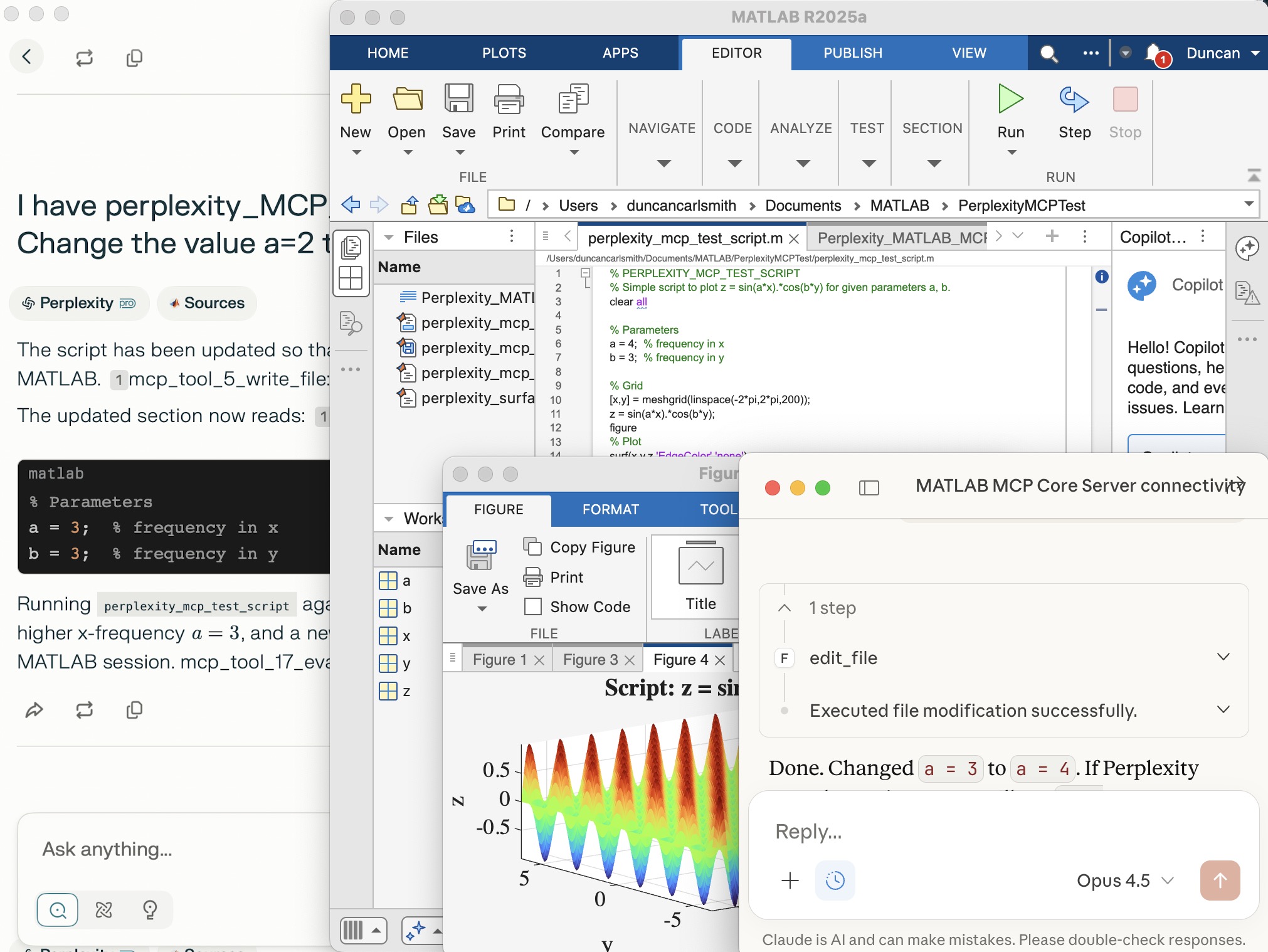
Note that Perplexity App’s file system access, like Claude App’s access, is limited to a folder of your choice, but both can issue system commands through MATLAB, so they inherit MATLAB’s privileges. Access can be restricted on a Mac by denying full disk access under Sytem Settings->Privacy and Security->Full Disk Access but that may be insufficient protection. Be careful. Also, when issuing a command to the MCP Server, both require you to review and approve any operation by default and allow you to override that behavior.
Screen sharing with Perplexity
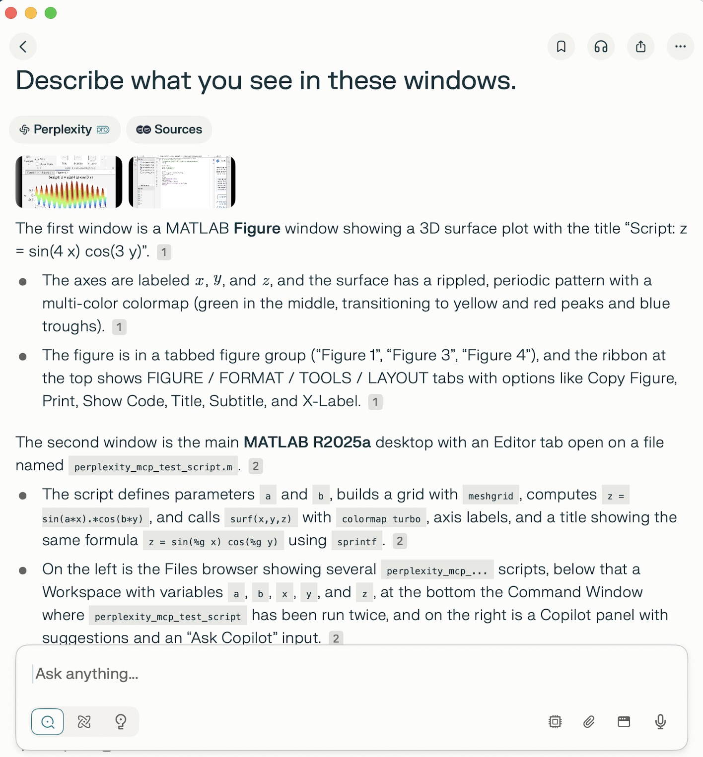
While Perplexity and Claude Apps do not “see” figures and other non-standard output via the MCP server unless saved to files the can access through its file server, Perplexity can in fact see the graphical results of a code and more through screen sharing, as demonstrated in the screenshot below of Perplexity App. At the bottom, below the Perplexity input form field, just to the left of the microphone, is a button enabling Perplexity to accept screen sharing from a selection of windows. I selected the MATLAB App window and the MATLAB Figure window and then asked Perplexity to describe the contents. Images of these wondows appear in the response as well as descriptions of the images. Sweet! No longer must I attempt to provide feedback by attempting to describe such results myself in words.
Appendix
(by Perplexity App)
Perplexity + MATLAB MCP Core Server Setup (macOS, R2025a)
1. Install and locate MATLAB
- Ensure MATLAB R2025a (or your chosen version) is installed under /Applications (e.g., /Applications/MATLAB_R2025a.app).
- From Terminal, verify MATLAB works:
"/Applications/MATLAB_R2025a.app/bin/matlab" -batch "ver"
This should list MATLAB and toolboxes without errors.
2. Fix PATH and shell alias for matlab
- Confirm the shell resolves the correct matlab:
which matlab
- If it is missing or points to an old version (e.g., R2022b), adjust:
export PATH="/Applications/MATLAB_R2025a.app/bin:$PATH"
which matlab
- Clear any stale alias or function:
type matlab
unalias matlab 2>/dev/null
unset -f matlab 2>/dev/null
which matlab
matlab -batch "ver"
Now matlab should invoke R2025a.
3. Place the MATLAB MCP Core Server binary
- Put the matlab-mcp-core-server binary in a convenient folder, e.g.:
/Users/duncancarlsmith/Developer/mcp-servers/matlab-mcp-core-server
- Make it executable:
cd /Users/duncancarlsmith/Developer/mcp-servers
chmod +x matlab-mcp-core-server
4. (Optional sanity check) Run the core server manually
- In Terminal, start the server once to confirm it can see MATLAB:
cd /Users/duncancarlsmith/Developer/mcp-servers
mkdir -p "$HOME/Claude-MATLAB-work"
./matlab-mcp-core-server \
--matlab-root="/Applications/MATLAB_R2025a.app" \
--initial-working-folder="$HOME/Claude-MATLAB-work"
- You should see INFO logs ending with:
"MATLAB MCP Core Server application startup complete".
- This process is not required long term once Perplexity is configured to launch the server itself.
5. Configure the MATLAB MCP connector in Perplexity (Mac app)
- Open Perplexity.
- Go to Settings → Connectors → Add Connector (or edit existing).
- Simple tab:
- Server command:
/Users/duncancarlsmith/Developer/mcp-servers/matlab-mcp-core-server --matlab-root /Applications/MATLAB_R2025a.app
- Advanced tab for the same connector:
{
"args": [
"--matlab-root",
"/Applications/MATLAB_R2025a.app"
],
"command": "/Users/duncancarlsmith/Developer/mcp-servers/matlab-mcp-core-server",
"env": {
},
"useBuiltInNode": true
}
- Save and ensure the connector shows as enabled.
6. Configure the filesystem MCP connector for MATLAB files
- Install the filesystem MCP server (one-time):
npx -y @modelcontextprotocol/server-filesystem /Users/duncancarlsmith/Documents/MATLAB
- In Perplexity Settings → Connectors → Add Connector:
- Name: filesystem (or similar).
- Server command:
npx -y @modelcontextprotocol/server-filesystem /Users/duncancarlsmith/Documents/MATLAB
- This allows Perplexity to list, create, and edit files directly under ~/Documents/MATLAB.
7. Test connectivity from Perplexity
- Start a new thread in Perplexity, with both the MATLAB connector and filesystem connector enabled.
- Verify MATLAB access by listing toolboxes or running a simple command via MCP:
- For example, list the contents of ~/Documents/MATLAB.
- Create a test folder (e.g., PerplexityMCPTest) using MATLAB or filesystem tools and confirm it appears.
8. Create and run a simple MATLAB script via Perplexity
- Using the filesystem connector, create a script in PerplexityMCPTest, e.g. perplexity_mcp_test_script.m:
% PERPLEXITY_MCP_TEST_SCRIPT
% Simple script to plot z = sin(a*x).*cos(b*y) for given parameters a, b.
clear all
% Parameters
a = 2; % frequency in x
b = 3; % frequency in y
% Grid
[x,y] = meshgrid(linspace(-2*pi,2*pi,200));
z = sin(a*x).*cos(b*y);
figure
% Plot
surf(x,y,z,'EdgeColor','none');
colormap turbo;
xlabel('x'); ylabel('y'); zlabel('z');
title(sprintf('Script: z = sin(%g x) cos(%g y)',a,b));
axis tight;
- From Perplexity, call MATLAB via the MCP server to run:
cd('PerplexityMCPTest'); perplexity_mcp_test_script
- In the local MATLAB desktop, a figure window will appear with the plotted surface.
9. Notes on behavior
- Perplexity interacts with MATLAB through the MCP Core Server and does not see the MATLAB GUI or figures; only text output/errors are visible to Perplexity.
- A brief extra MATLAB window may appear and disappear when the core server starts or manages its own MATLAB session; this is expected and separate from your own interactive MATLAB instance.
- File creation and editing from Perplexity occur via the filesystem MCP server and are limited to the configured root (here, ~/Documents/MATLAB).

% Recreation of Saturn photo
figure('Color', 'k', 'Position', [100, 100, 800, 800]);
ax = axes('Color', 'k', 'XColor', 'none', 'YColor', 'none', 'ZColor', 'none');
hold on;
% Create the planet sphere
[x, y, z] = sphere(150);
% Saturn colors - pale yellow/cream gradient
saturn_radius = 1;
% Create color data based on latitude for gradient effect
lat = asin(z);
color_data = rescale(lat, 0.3, 0.9);
% Plot Saturn with smooth shading
planet = surf(x*saturn_radius, y*saturn_radius, z*saturn_radius, ...
color_data, ...
'EdgeColor', 'none', ...
'FaceColor', 'interp', ...
'FaceLighting', 'gouraud', ...
'AmbientStrength', 0.3, ...
'DiffuseStrength', 0.6, ...
'SpecularStrength', 0.1);
% Use a cream/pale yellow colormap for Saturn
cream_map = [linspace(0.4, 0.95, 256)', ...
linspace(0.35, 0.9, 256)', ...
linspace(0.2, 0.7, 256)'];
colormap(cream_map);
% Create the ring system
n_points = 300;
theta = linspace(0, 2*pi, n_points);
% Define ring structure (inner radius, outer radius, brightness)
rings = [
1.2, 1.4, 0.7; % Inner ring
1.45, 1.65, 0.8; % A ring
1.7, 1.85, 0.5; % Cassini division (darker)
1.9, 2.3, 0.9; % B ring (brightest)
2.35, 2.5, 0.6; % C ring
2.55, 2.8, 0.4; % Outer rings (fainter)
];
% Create rings as patches
for i = 1:size(rings, 1)
r_inner = rings(i, 1);
r_outer = rings(i, 2);
brightness = rings(i, 3);
% Create ring coordinates
x_inner = r_inner * cos(theta);
y_inner = r_inner * sin(theta);
x_outer = r_outer * cos(theta);
y_outer = r_outer * sin(theta);
% Front side of rings
ring_x = [x_inner, fliplr(x_outer)];
ring_y = [y_inner, fliplr(y_outer)];
ring_z = zeros(size(ring_x));
% Color based on brightness
ring_color = brightness * [0.9, 0.85, 0.7];
fill3(ring_x, ring_y, ring_z, ring_color, ...
'EdgeColor', 'none', ...
'FaceAlpha', 0.7, ...
'FaceLighting', 'gouraud', ...
'AmbientStrength', 0.5);
end
% Add some texture/gaps in the rings using scatter
n_particles = 3000;
r_particles = 1.2 + rand(1, n_particles) * 1.6;
theta_particles = rand(1, n_particles) * 2 * pi;
x_particles = r_particles .* cos(theta_particles);
y_particles = r_particles .* sin(theta_particles);
z_particles = (rand(1, n_particles) - 0.5) * 0.02;
% Vary particle brightness
particle_colors = repmat([0.8, 0.75, 0.6], n_particles, 1) .* ...
(0.5 + 0.5*rand(n_particles, 1));
scatter3(x_particles, y_particles, z_particles, 1, particle_colors, ...
'filled', 'MarkerFaceAlpha', 0.3);
% Add dramatic outer halo effect - multiple layers extending far out
n_glow = 20;
for i = 1:n_glow
glow_radius = 1 + i*0.35; % Extend much farther
alpha_val = 0.08 / sqrt(i); % More visible, slower falloff
% Color gradient from cream to blue/purple at outer edges
if i <= 8
glow_color = [0.9, 0.85, 0.7]; % Warm cream/yellow
else
% Gradually shift to cooler colors
mix = (i - 8) / (n_glow - 8);
glow_color = (1-mix)*[0.9, 0.85, 0.7] + mix*[0.6, 0.65, 0.85];
end
surf(x*glow_radius, y*glow_radius, z*glow_radius, ...
ones(size(x)), ...
'EdgeColor', 'none', ...
'FaceColor', glow_color, ...
'FaceAlpha', alpha_val, ...
'FaceLighting', 'none');
end
% Add extensive glow to rings - make it much more dramatic
n_ring_glow = 12;
for i = 1:n_ring_glow
glow_scale = 1 + i*0.15; % Extend farther
alpha_ring = 0.12 / sqrt(i); % More visible
for j = 1:size(rings, 1)
r_inner = rings(j, 1) * glow_scale;
r_outer = rings(j, 2) * glow_scale;
brightness = rings(j, 3) * 0.5 / sqrt(i);
x_inner = r_inner * cos(theta);
y_inner = r_inner * sin(theta);
x_outer = r_outer * cos(theta);
y_outer = r_outer * sin(theta);
ring_x = [x_inner, fliplr(x_outer)];
ring_y = [y_inner, fliplr(y_outer)];
ring_z = zeros(size(ring_x));
% Color gradient for ring glow
if i <= 6
ring_color = brightness * [0.9, 0.85, 0.7];
else
mix = (i - 6) / (n_ring_glow - 6);
ring_color = brightness * ((1-mix)*[0.9, 0.85, 0.7] + mix*[0.65, 0.7, 0.9]);
end
fill3(ring_x, ring_y, ring_z, ring_color, ...
'EdgeColor', 'none', ...
'FaceAlpha', alpha_ring, ...
'FaceLighting', 'none');
end
end
% Add diffuse glow particles for atmospheric effect
n_glow_particles = 8000;
glow_radius_particles = 1.5 + rand(1, n_glow_particles) * 5;
theta_glow = rand(1, n_glow_particles) * 2 * pi;
phi_glow = acos(2*rand(1, n_glow_particles) - 1);
x_glow = glow_radius_particles .* sin(phi_glow) .* cos(theta_glow);
y_glow = glow_radius_particles .* sin(phi_glow) .* sin(theta_glow);
z_glow = glow_radius_particles .* cos(phi_glow);
% Color particles based on distance - cooler colors farther out
particle_glow_colors = zeros(n_glow_particles, 3);
for i = 1:n_glow_particles
dist = glow_radius_particles(i);
if dist < 3
particle_glow_colors(i,:) = [0.9, 0.85, 0.7];
else
mix = (dist - 3) / 4;
particle_glow_colors(i,:) = (1-mix)*[0.9, 0.85, 0.7] + mix*[0.5, 0.6, 0.9];
end
end
scatter3(x_glow, y_glow, z_glow, rand(1, n_glow_particles)*2+0.5, ...
particle_glow_colors, 'filled', 'MarkerFaceAlpha', 0.05);
% Lighting setup
light('Position', [-3, -2, 4], 'Style', 'infinite', ...
'Color', [1, 1, 0.95]);
light('Position', [2, 3, 2], 'Style', 'infinite', ...
'Color', [0.3, 0.3, 0.4]);
% Camera and view settings
axis equal off;
view([-35, 25]); % Angle to match saturn_photo.jpg - more dramatic tilt
camva(10); % Field of view - slightly wider to show full halo
xlim([-8, 8]); % Expanded to show outer halo
ylim([-8, 8]);
zlim([-8, 8]);
% Material properties
material dull;
title('Saturn - Left click: Rotate | Right click: Pan | Scroll: Zoom', 'Color', 'w', 'FontSize', 12);
% Enable interactive camera controls
cameratoolbar('Show');
cameratoolbar('SetMode', 'orbit'); % Start in rotation mode

% Custom mouse controls
set(gcf, 'WindowButtonDownFcn', @mouseDown);
function mouseDown(src, ~)
selType = get(src, 'SelectionType');
switch selType
case 'normal' % Left click - rotate
cameratoolbar('SetMode', 'orbit');
rotate3d on;
case 'alt' % Right click - pan
cameratoolbar('SetMode', 'pan');
pan on;
end
end