Working with Quantile Regression Models

Quantile regression models allow you to model the conditional distribution of a response variable, given the value of predictor variables. You can use a fitted model to estimate quantiles (quantile) in the conditional distribution of the response. Also, you can use quantile regression models to estimate prediction intervals and fit models that are robust to outliers. For examples, see Create Prediction Interval Using Quantiles and Fit Regression Models to Data with Outliers.

You can perform quantile regression in Statistics and Machine Learning Toolbox™ using linear models, neural networks, or bagged ensembles.

• fitrqlinear — Train a quantile linear regression model. Use the predict and loss object functions of the resulting RegressionQuantileLinear object.

• fitrqnet — Train a regression quantile neural network. Use the predict and loss object functions of the resulting RegressionQuantileNeuralNetwork object.

• TreeBagger — Train a bag of regression trees (or random forest). Use the quantilePredict and quantileError object functions of the resulting TreeBagger object.

When using linear and neural network models to perform quantile regression, consider using regularization to prevent quantile crossing. For more information, see Regularize Quantile Regression Model to Prevent Quantile Crossing.

Create Prediction Interval Using Quantiles

Train a linear regression model. Use the 0.05 and 0.95 quantiles of the response to create a prediction interval that captures an estimated 90% of the variation in the response.

Generate 1000 observations from the model$$y=1+0.01x+(0.02x)ϵ$$.

• The predictor values (x) are evenly spaced between 0 and 10.

• The error values ($$ϵ$$) are uniformly distributed in the interval (0,1).

• y is the response.

rng("default"); % For reproducibility
n = 1000;
x = linspace(0,10,n)';
y = 1 + (0.01 + 0.2*rand(n,1)).*x;

Train a regression model using the data in x and y. Then, generate 250 test set values of predictor data, evenly spaced between 0 and 10, and use the regression model to predict the response for the test data.

Mdl = fitrlinear(x,y);
xPred = linspace(0,10,250)';
yPred = predict(Mdl,xPred);

Visualize the predictions along with the training data.

figure
plot(x,y,".")
hold on
plot(xPred,yPred,LineWidth=1)
hold off
xlabel("x")
ylabel("y")
legend(["Training data","Mean predictions (test data)"],Location="northwest")

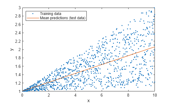
The blue points correspond to the training observations, and the red line corresponds to the predictions for the test data. At each fixed predictor value, the red line shows the mean response, but it does not indicate the variation in the response.

To capture the variation in the response, create a 90% prediction interval by using a quantile regression model. Specify to use the 0.05 and 0.95 quantiles.

quantileMdl = fitrqlinear(x,y,Quantiles=[0.05 0.95]);

Use the quantile regression model to predict the 0.05 and 0.95 quantile responses for the test data.

yInt = predict(quantileMdl,xPred);

Add the quantile predictions to the previous plot.

figure
plot(x,y,".")
hold on
plot(xPred,yPred,LineWidth=1)
plot(xPred,yInt(:,1),LineWidth=1)
plot(xPred,yInt(:,2),LineWidth=1)
xlabel("x")
ylabel("y")
legend(["Training data","Mean predictions (test data)", ...
    "0.05 quantile predictions (test data)", ...
    "0.95 quantile predictions (test data)"], ...
    Location="northwest")
hold off

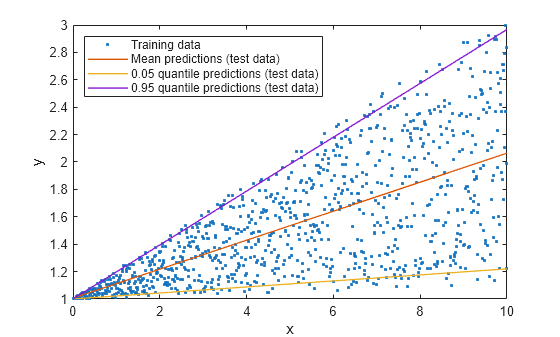
The yellow and purple lines form a prediction interval that contains an estimated 90% of the variation in the response.

For a more in-depth example that shows how to create prediction intervals with validity guarantees, see Create Prediction Intervals Using Split Conformal Prediction.

Fit Regression Models to Data with Outliers

Compare a neural network regression model that estimates the mean response to a quantile neural network model that estimates the median response. Because the median is less influenced by outliers than the mean, using the fitrqnet function can be a good alternative to using the fitrnet function when fitting a neural network model to data with outliers.

Generate 200 observations from the model $\mathit{y}=1+0.05\mathit{x}+\frac{\sin \left(\mathit{x}\right)}{\mathit{x}}+ϵ$.

• The predictor values (x) are evenly spaced between –10 and 10.

• The error values ($ϵ$) follow the normal distribution with mean 0 and standard deviation 0.2.

• y is the response.

rng("default"); % For reproducibility
n = 200;
x = linspace(-10,10,n)';
y = 1 + 0.05*x + sin(x)./x + 0.2*randn(n,1);

For this example, add three outliers to the data.

x(201:203) = [-5 0 7.5];
y(201:203) = [2 0.5 0.5];

Train a neural network regression model using the data in x and y (including outliers).

meanMdl = fitrnet(x,y)

meanMdl = 
  RegressionNeuralNetwork
             ResponseName: 'Y'
    CategoricalPredictors: []
        ResponseTransform: 'none'
          NumObservations: 203
               LayerSizes: 10
              Activations: 'relu'
    OutputLayerActivation: 'none'
                   Solver: 'LBFGS'
          ConvergenceInfo: [1×1 struct]
          TrainingHistory: [510×7 table]


  Properties, Methods

meanMdl is a RegressionNeuralNetwork model object.

For comparison, train a quantile neural network regression model using the same training data. By default, the model uses the median (or 0.5 quantile) to estimate the response.

medianMdl = fitrqnet(x,y)

medianMdl = 
  RegressionQuantileNeuralNetwork
             ResponseName: 'Y'
    CategoricalPredictors: []
               LayerSizes: 10
              Activations: 'relu'
    OutputLayerActivation: 'none'
                Quantiles: 0.5000


  Properties, Methods

medianMdl is a RegressionQuantileNeuralNetwork model object.

To see the difference in behavior between the two models, generate 100 observations of predictor data, evenly spaced between –10 and 10. Use the two neural network models to predict the response for the observations.

predX = linspace(-10,10,100)';
meanPredY = predict(meanMdl,predX);
medianPredY = predict(medianMdl,predX);

Visualize the predictions along with the training data.

plot(x,y,".")
hold on
plot(predX,meanPredY)
plot(predX,medianPredY)
hold off
legend(["Training data","Mean model","Median model"])

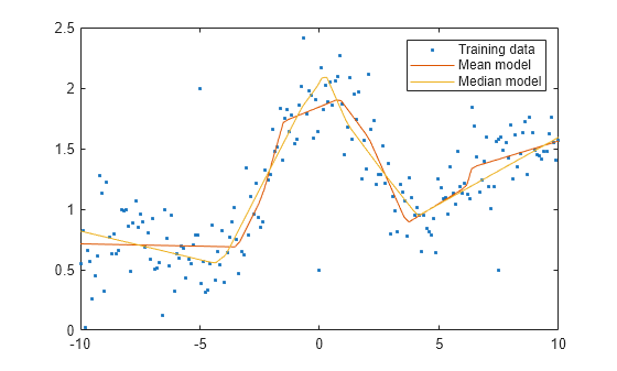
Recall that the outliers are located at (–5,2), (0,0.5), and (7.5,0.5). The plot suggests that the neural network model meanMdl, with predictions in red, is influenced by these outliers. For example, the prediction curve flattens for values of x around 0. The quantile neural network model medianMdl, with predictions in yellow, seems to be more robust to the outliers.