Regularize Quantile Regression Model to Prevent Quantile Crossing

This example shows how to regularize a quantile regression model to prevent quantile crossing. You can use quantile regression to create prediction intervals in workflows for uncertainty estimation and AI verification. Quantile crossing can negatively affect these workflows by returning invalid prediction intervals. For an example that shows how to create prediction intervals for uncertainty estimation, see Create Prediction Interval Using Quantiles.

Introduction

Quantile crossing, a limitation of some quantile regression approaches, occurs when estimated quantiles are not monotonic in the quantile values. According to the monotonicity property, if quantile ${\tau }_1$ is less than quantile ${\tau }_2$, then the prediction corresponding to ${\tau }_1$ must be less than or equal to the prediction corresponding to ${\tau }_2$. The quantile crossing problem occurs when the monotonicity property is not satisfied.

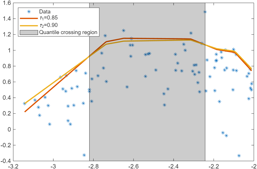
The plot below shows two quantile estimates corresponding to the quantiles 0.85 and 0.90. The gray region shows where the monotonicity property is not satisfied and the quantile crossing problem occurs.

Regularizing the quantile regression model is an effective approach for reducing the likelihood of quantile crossing. This example demonstrates the effectiveness of regularization using the following steps:

1. Generate data from a linear model with heteroscedastic error.

2. Train quantile linear regression models with various regularization strengths using cross-validation.

3. Choose the optimal regularization strength that results in no quantile crossing.

4. Train a final quantile linear regression model with the optimal regularization strength.

Generate Data

Consider the following linear model with heteroscedastic error, discussed in [1]:

$$y(i)={\beta }_0+\sum _{j=1}^p{\beta }_j{X}_j(i)+({\gamma }_0+\sum _{j=1}^p{\gamma }_j{X}_j(i))ϵ(i)$$

• $$X$$ is the predictor data, an n-by-p matrix of uniformly distributed values in the range (0,1). n is the number of observations, and p is the number of predictors. $$X_j(i)$$ is the predictor value $$j$$ for observation $$i$$.

• $$ϵ$$ is an n-by-1 vector of standard normal error values, where $$ϵ(i)$$ is the error value for observation $$i$$.

• $$\beta =({\beta }_0,...,{\beta }_p)$$ are model coefficients, and $$\gamma =({\gamma }_0,...,{\gamma }_p)$$ are coefficients for the error term.

• $$y(i)$$ is the response for observation $$i$$.

Generate 500 observations from the linear model with $$\beta =(1,1,1,1,1,1,1,1)$$ and $$\gamma =(1,1,1,1,0,0,0,0)$$. Note that the model has $\mathit{p}=7$ predictors.

n = 500;
p = 7;
beta0 = 1;
gamma0 = 1;
beta = [1 1 1 1 1 1 1];
gamma = [1 1 1 0 0 0 0];

rng(0,"twister"); % For reproducibility
X = rand(n,p);
epsilon = normrnd(0,1,n,1);
y = beta0 + X*beta' + (gamma0 + X*gamma').*epsilon;

X contains the predictor data, and y contains the response variable.

Create a set of 10 logarithmically spaced regularization strengths from ${10}^{-4}$ to ${10}^{-1}$.

maxLambda = 0.1;
numLambda = 10;
lambda = [logspace(log10(maxLambda/1000), ...
    log10(maxLambda),numLambda)];

lambda contains the regularization strengths.

Train Quantile Linear Regression Models

First, create a default quantile linear regression model using the data in X and y. Specify to use the 0.85, 0.90, and 0.95 quantiles.

quantiles = [0.85,0.9,0.95];
firstMdl = fitrqlinear(X,y,Quantiles=quantiles);

Use 5-fold cross-validation to determine the number of observations that have crossing quantile predictions when the observations are in a test set.

firstValidationMdl = crossval(firstMdl,KFold=5);
[~,crossingIndicator] = kfoldPredict(firstValidationMdl);
sum(crossingIndicator)

ans = 
9

The quantile predictions returned by the model cross for 9 of the observations.

Check the regularization strength used in firstMdl.

firstMdl.Lambda

ans = 
0.0020

By default, fitrqlinear uses a regularization strength of approximately 1/n, where n is the number of training observations.

To prevent quantile crossing in the model, adjust the regularization strength. A greater regularization strength in a linear model penalizes larger coefficient values, resulting in a smoother model. Smoother models produce more consistent quantile estimates, which reduces the likelihood of quantile crossing.

To determine the optimal regularization strength to use, train a quantile regression model for each regularization strength in lambda. Use 5-fold cross-validation to find the regularized model that returns the smallest quantile loss with no quantile crossing.

numQuantiles = numel(quantiles);
numCrossings = zeros(numLambda,1);
lossVals = zeros(numLambda,numQuantiles);
for i = 1:numLambda
    mdl = fitrqlinear(X,y,Quantiles=quantiles,Lambda=lambda(i),KFold=5);
    [~,isIndicator] = kfoldPredict(mdl);
    lossVals(i,:)= kfoldLoss(mdl);
    numCrossings(i) = sum(isIndicator);
end

Plot the number of observations with quantile predictions that cross for each regularized model.

figure
plot(log10(lambda),numCrossings,Marker="o")
ylabel("Number of Points with Crossings")
xlabel("log_{10} of Lambda")

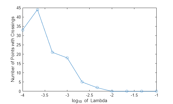
The plot shows that the number of observations with quantile predictions that cross is 0 for the cross-validated models with regularization strengths between ${10}^{-2}$ and ${10}^{-1}$.

Choose Optimal Regularization Strength

Find the regularization strength in lambda that results in the lowest quantile loss while producing no quantile crossing. A lower quantile loss corresponds to better model accuracy.

Inspect the loss values for the cross-validated models.

lossVals

lossVals = 10×3

    0.5693    0.4191    0.2492
    0.5756    0.4265    0.2540
    0.5713    0.4255    0.2535
    0.5675    0.4261    0.2542
    0.5641    0.4226    0.2538
    0.5721    0.4351    0.2683
    0.5879    0.4495    0.2772
    0.6043    0.4681    0.2872
    0.6116    0.4703    0.2872
    0.6198    0.4780    0.2941

lossVals contains the average quantile loss values for the cross-validated models. The rows correspond to models, and the columns correspond to quantiles. For example, lossVals(5,3) contains the quantile loss for quantiles(3), averaged across all folds, of the cross-validated model with regularization strength lambda(5).

For each model, compute the sum of the quantile loss values for the three quantiles (0.85, 0.90, and 0.95).

quantileLossSum = sum(lossVals,2);

For each log-transformed regularization strength, plot the number of observations with quantile predictions that cross (in blue) and the log-transformed sum of quantile losses (in red).

figure
yyaxis left
plot(log10(lambda),numCrossings,Marker="o")
ylabel("Number of Points with Crossings")

yyaxis right
plot(log10(lambda),log10(quantileLossSum),Marker="o")
ylabel("log_{10} of the Sum of Quantile Losses")

xlabel("log_{10} of Lambda")
legend(["Num points with crossings","Log of quantile loss sum"], ...
    Location="north")

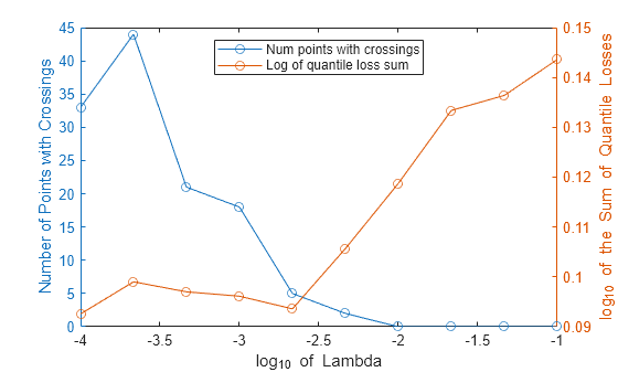
In this example, the optimal lambda value is the one where the blue curve is 0 and the red curve is as low as possible. In general, you can choose to minimize a different loss criterion (that is, a different red curve).

Find the optimal regularization strength programmatically.

noCrossingsIdx = (numCrossings == 0);
noCrossingsLossVals = lossVals(noCrossingsIdx,:);
noCrossingsLambda = lambda(noCrossingsIdx);

[~,minIdx] = min(sum(noCrossingsLossVals,2));
optimalLambda = noCrossingsLambda(minIdx)

optimalLambda = 
0.0100

The optimal regularization strength is ${10}^{-2}$.

Train Final Quantile Regression Model

Train a quantile linear regression model with the optimal regularization strength. Use 5-fold cross-validation to confirm that no observations have quantile predictions that cross.

finalMdl = fitrqlinear(X,y,Quantiles=quantiles,Lambda=optimalLambda);

finalValidationMdl = crossval(finalMdl,KFold=5);
[~,finalCrossingIndicator] = kfoldPredict(finalValidationMdl);
sum(finalCrossingIndicator)

ans = 
0

finalMdl is a quantile linear regression model that has been regularized to prevent quantile crossing over the simulated data.

Conclusion

You can use regularization to prevent quantile crossing for linear and neural network quantile regression models (created using fitrqlinear and fitrqnet, respectively). Although regularization is effective at preventing quantile crossing, the technique does not guarantee the absence of crossing quantile predictions over unseen data. Check carefully for quantile crossing when the monotonicity of the quantile estimates is a requirement over unseen data.

If the absence of quantile crossing over unseen data must be guaranteed, you can use quantile random forests instead. Use the TreeBagger function to create a random forest of regression trees, and then use quantilePredict to predict response quantiles. Quantile random forests ensure that ${\tau }_1$ quantile estimates are less than or equal to ${\tau }_2$ quantile estimates for ${\tau }_1<{\tau }_2$. For more information, see [2].

References

[1] Bondell, H. D., B. J. Reich, and H. Wang. "Noncrossing Quantile Regression Curve Estimation." Biometrika 97, no. 4 (2010): 825–38.

[2] Meinshausen, Nicolai. "Quantile Regression Forests." Journal of Machine Learning Research 7 (2006): 983–99.