Create Prediction Intervals Using Split Conformal Prediction

This example shows how to create prediction intervals using split conformal prediction. Split conformal prediction, or SCP, is a distribution-free, model-agnostic statistical framework that returns prediction intervals with validity guarantees, given an acceptable error rate. This example uses a popular SCP technique called "conformalized quantile regression." For more information, see [1].

In general, prediction intervals estimate the spread of the true response. You can use this information to assess the uncertainty associated with a regression model and its predictions. Uncertainty estimation is important in safety critical applications, where the AI system must be able to generalize over unseen data, and the uncertainty associated with the AI model predictions must be handled in a way that does not compromise safety.

This example includes the following steps:

1. Generate data from a nonlinear model with heteroscedasticity.

2. Partition the generated data into a training set, a calibration set, and a test set.

3. Train a quantile neural network model using the training set.

4. Compute a 90% prediction interval for the test observations. Use conformalized quantile regression to calibrate the prediction interval.

5. Assess the performance of the prediction interval on the test set.

For more information on SCP, see Split Conformal Prediction.

Generate Data

Generate 20,000 observations from this nonlinear model with heteroscedastic error: $$y=10+3x+x\sin (2x)+ϵ\sqrt{(x+0.1)}$$.

• x is an n-by-1 predictor variable, where n is the number of observations. The values are randomly selected, with replacement, from a set of 1,000,000 evenly spaced values between 0 and $$4\pi$$.

• $$ϵ$$ is an n-by-1 vector of standard normal values. The $$ϵ\sqrt{(x+0.1)}$$ term corresponds to the heteroscedastic error of the model.

• y is the n-by-1 response variable.

n = 20000;
rng(2,"twister"); % For reproducibility
x = randsample(linspace(0,4*pi,1e6),n,true)';
epsilon = randn(n,1);
y = 10 + 3*x + x.*sin(2*x) + epsilon.*sqrt(x+0.01);

Partition Data

Partition the generated data into two sets: one for testing and one for training and calibration. Reserve 20% of the observations for the test set, and count the number of observations in the test set.

cv1 = cvpartition(n,Holdout=0.20);

xSCP = x(cv1.training,:);
ySCP = y(cv1.training,:);

xTest = x(cv1.test,:);
yTest = y(cv1.test,:);
numTest = numel(xTest);

Sort the test observations so that the predictor values are in ascending order.

[xTest,idx] = sort(xTest);
yTest = yTest(idx);

Now partition the remaining observations into two sets of approximately the same size. The first set of data (xTrain and yTrain) is for training a quantile regression model, from which you can create a prediction interval with the test data. The second set of data (xCalibration and yCalibration) is for calibrating the prediction interval. Count the number of observations in the calibration set.

cv2 = cvpartition(cv1.TrainSize,Holdout=0.50);

xTrain = xSCP(cv2.training,:);
yTrain = ySCP(cv2.training,:);

xCalibration = xSCP(cv2.test,:);
yCalibration = ySCP(cv2.test,:);
numCalibration = numel(xCalibration);

Train Quantile Neural Network Model

Before training a quantile regression model, set the acceptable error rate $\alpha$ to 0.1. When you create a prediction interval, the acceptable error rate is the proportion of true response values that are allowed to fall outside of the prediction interval.

Train a quantile neural network model using the data in xTrain and yTrain. Use the quantiles $$\alpha /2=0.05$$ and $$1-\alpha /2=0.95$$. Specify to standardize the predictor data, and to have 50 outputs in both the first and second fully connected layers of the neural network.

alpha = 0.1;
quantileMdl = fitrqnet(xTrain,yTrain,Quantiles=[alpha/2 1-alpha/2], ...
    Standardize=true,LayerSizes=[50 50])

quantileMdl = 
  RegressionQuantileNeuralNetwork
             ResponseName: 'Y'
    CategoricalPredictors: []
               LayerSizes: [50 50]
              Activations: 'relu'
    OutputLayerActivation: 'none'
                Quantiles: [0.0500 0.9500]


  Properties, Methods

quantileMdl is a RegressionQuantileNeuralNetwork model object. You can use the model to make quantile predictions on new data.

Compute Prediction Interval

To compute a prediction interval for the test observations, first compute conformity scores for the calibration observations, as defined in conformalized quantile regression [1]. Then, derive a score quantile from the conformity scores. Finally, compute and calibrate the prediction interval.

Create the custom conformityScores function. The function accepts a quantile regression model (Mdl) with quantiles $$\alpha /2$$ and $$1-\alpha /2$$, predictor data (x), and response data (y). For each observation, the function returns a conformity score, which is the maximum of the following values:

• The difference between the $$\alpha /2$$ quantile model prediction and the true response

• The difference between the true response and the $$1-\alpha /2$$ quantile model prediction

function scores = conformityScores(Mdl,x,y)
predictions = predict(Mdl,x);
r = [predictions(:,1) - y, y - predictions(:,2)];
scores = max(r,[],2);
end

Compute the conformity scores using the trained quantile neural network model quantileMdl and the data in xCalibration and yCalibration.

s = conformityScores(quantileMdl,xCalibration,yCalibration);

Calculate the score quantile to use for calibrating the prediction interval.

p = (1+1/numCalibration)*(1-alpha);
q = quantile(s,p)

q = 
0.0476

Compute the 90% prediction interval for the data in xTest. First, use the predict function of the trained quantile model to return 0.05 and 0.95 quantile predictions for the test data. Then, adjust the predictions by using the score quantile q.

quantilePredictions = predict(quantileMdl,xTest);
yint = [quantilePredictions(:,1) - q, quantilePredictions(:,2) + q];

yint(:,1) corresponds to the lower bound of the prediction interval, and yint(:,2) corresponds to the upper bound of the prediction interval.

Assess Prediction Interval

You can assess prediction intervals for statistical efficiency by computing their miscoverage rate. The average miscoverage is the proportion of test set observations that have true response values outside of the prediction interval.

Find the average miscoverage rate for yint. Confirm that this rate is less than the acceptable error rate $\alpha$.

averageMiscoverage = nnz(yTest < yint(:,1) | yTest > yint(:,2))/numTest

averageMiscoverage = 
0.0965

averageMiscoverage is less than 0.1, the value of the acceptable error rate.

Plot the test data and the prediction interval.

figure
scatter(xTest,yTest,"filled")
hold on
plot(xTest,yint,LineWidth=3,Color=[0.4940 0.1840 0.5560])
hold off
legend(["Test data","Prediction interval",""], ...
    Location="northwest")
xlabel("x")
ylabel("y")
title("Prediction Intervals Obtained Using SCP")

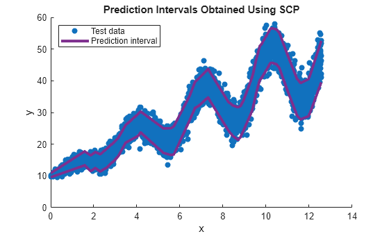
The plot shows that the prediction interval adapts to the heteroscedasticity of the data. That is, the prediction interval is smaller in regions of lower response spread, and larger in regions of higher response spread.

References

[1] Romano, Yaniv, Evan Patterson, and Emmanuel Candes. "Conformalized Quantile Regression." Advances in Neural Information Processing Systems 32 (2019).