Perform Incremental Learning Using IncrementalClassificationECOC Fit and Predict Blocks

Since R2024a

This example shows how to use the IncrementalClassificationECOC Predict and IncrementalClassificationECOC Fit blocks for incremental learning and classification in Simulink®. The IncrementalClassificationECOC Fit block fits a chunk of observations (predictor data) using a configured incremental multiclass ECOC classification model (incrementalClassificationECOC) and outputs updated incremental learning model parameters as a bus signal. The IncrementalClassificationECOC Predict block accepts an IncrementalClassificationECOC model and a chunk of predictor data, and returns the predicted class label, class scores, and positive-class scores of binary learners.

Load Data

Load the humanactivity data set and randomly shuffle the data.

load humanactivity
n = numel(actid);
rng(0,"twister") % For reproducibility
idx = randsample(n,n);
X = feat(idx,:);
Y = actid(idx);

The numeric matrix X contains 24,075 observations of five physical human activities. Each observation has 60 features extracted from acceleration data measured by smartphone accelerometer sensors. The numeric matrix Y contains the activity IDs in integers: 1, 2, 3, 4, and 5 representing sitting, standing, walking, running, and dancing, respectively.

Create Incremental Learning Model

Create an incremental multiclass ECOC classification model and specify to use one-versus-all coding. Also specify that the data has 60 predictors and class labels 1, 2, 3, 4, and 5. Create a workspace variable ecocMdl to store the initial incremental learning model.

Mdl = incrementalClassificationECOC(coding="onevsall", ...
    NumPredictors=60,ClassNames=[1,2,3,4,5]);
ecocMdl = Mdl;

ecocMdl is an incrementalClassificationECOC model. You can use dot notation to access the properties of ecocMdl. For example, enter ecocMdl.CodingMatrix to display the coding design matrix of the model.

ecocMdl.CodingMatrix

ans = 5×5

     1    -1    -1    -1    -1
    -1     1    -1    -1    -1
    -1    -1     1    -1    -1
    -1    -1    -1     1    -1
    -1    -1    -1    -1     1

Each row of the coding design matrix corresponds to a class, and each column corresponds to a binary learner.

Enter ecocMdl.BinaryLearners to display the model type of each binary learner.

ecocMdl.BinaryLearners

ans=5×1 cell array
    {1x1 incrementalClassificationLinear}
    {1x1 incrementalClassificationLinear}
    {1x1 incrementalClassificationLinear}
    {1x1 incrementalClassificationLinear}
    {1x1 incrementalClassificationLinear}

Enter ecocMdl.BinaryLoss to display the binary learner loss function.

ecocMdl.BinaryLoss

ans = 
'hinge'

To classify a new observation, the model computes positive-class classification scores for the binary learners, applies the hinge function to the scores to compute the binary losses, and then combines the binary losses into the classification scores using the loss-weighted decoding scheme.

Create Input Data for Simulink

Simulate streaming data by dividing the training data into chunks of 50 observations. For each chunk, select a single observation as a test set to import into the IncrementalClassificationECOC Predict block.

numObsPerChunk = 50;
nchunk = floor(n/numObsPerChunk);
for j = 1:nchunk
    ibegin = min(n,numObsPerChunk*(j-1) + 1);
    iend   = min(n,numObsPerChunk*j);
    idx = ibegin:iend;   
    Mdl = fit(Mdl,X(idx,:),Y(idx));    
    Xin(:,:,j) = X(idx,:);
    Yin(:,j) = Y(idx);
    Xtest(1,:,j) = X(idx(1),:);
 end

Convert the training and test set chunks into time series objects.

t = 0:size(Xin,3)-1;
Xtrain_ts = timeseries(Xin,t,'InterpretSingleRowDataAs3D',true);
Ytrain_ts = timeseries(Yin',t,'InterpretSingleRowDataAs3D',true);
Xtest_ts = timeseries(Xtest,t,'InterpretSingleRowDataAs3D',true);

Open Provided Simulink Model

This example provides the Simulink model slexIncClassificationECOCPredictExample.slx, which includes the IncrementalClassificationECOC Predict and IncrementalClassificationECOC Fit blocks. The Simulink model is configured to use ecocMdl as the initial model for incremental learning and classification.

Open the Simulink model slexIncClassificationECOCPredictExample.slx.

slName = "slexIncClassificationECOCPredictExample";
open_system(slName)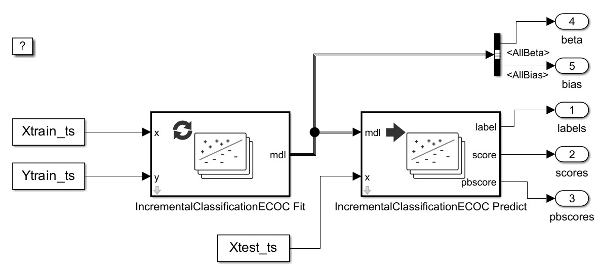

Simulate Model

Simulate the Simulink model to perform incremental learning and predict responses to the test set observations. Export the simulation outputs to the workspace. You can use the Simulation Data Inspector (Simulink) to view the logged data of an Outport block.

simOut = sim(slName,"StopTime",num2str(numel(t)-1));
% Extract labels
label_sig = simOut.yout.getElement(1);
label_sl = squeeze(label_sig.Values.Data);

% Extract score values
score_sig = simOut.yout.getElement(2);
score_sl = squeeze(score_sig.Values.Data);

% Extract positive class score values
pbscore_sig = simOut.yout.getElement(3);
pbscore_sl = squeeze(pbscore_sig.Values.Data);

% Extract beta values
beta_sig = simOut.yout.getElement(4);
beta_sl = squeeze(beta_sig.Values.Data);

% Extract bias values
bias_sig = simOut.yout.getElement(5);
bias_sl = squeeze(bias_sig.Values.Data);

At each iteration, the IncrementalClassificationECOC Fit block trains the model and updates the model parameters. The IncrementalClassificationECOC Predict block calculates the predicted label for the test set observation.

Analyze Model During Training

Plot the model parameters and model performance values for each data chunk on separate tiles.

figure
tiledlayout(5,1);
nexttile
plot(label_sl,".")
ylabel("Label")
xlabel("Iteration")
xlim([0 nchunk])
nexttile
plot(score_sl(1,:),".")
ylabel("Score")
xlabel("Iteration")
xlim([0 nchunk])
nexttile
plot(pbscore_sl(1,:),".-")
ylabel("PB Score")
xlabel("Iteration")
xlim([0 nchunk])
nexttile
plot(squeeze(beta_sl(1,1,:)),".-")
ylabel("\beta_1")
xlabel("Iteration")
xlim([0 nchunk])
nexttile
plot(bias_sl(:,1),".-")
ylabel("Bias (1)")
xlabel("Iteration")
xlim([0 nchunk])

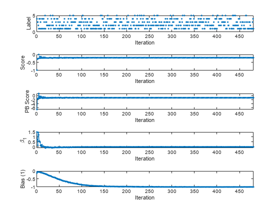
During incremental learning, the score of the first class has an initial value of –1, and then rapidly approaches –0.2. The positive-class score of the first class has an initial value of –6.7, and then rapidly approaches –1. The first beta coefficient of the first binary learner initially fluctuates between 0.15 and 1.5, and then approaches 0. The bias (intercept) term of the first binary learner has an initial value of –0.13, and then gradually approaches –1.