Sliding Mode Control of DC Motor

Since R2025a

This example show how to use the Linear Sliding Mode Controller (State Feedback) block such that the DC motor position tracks a square wave reference signal.

DC Motor Implementation

The DC motor is modeled using Simscape™, which provides a realistic simulation environment. The motor in this example is based on the Maxon: RE 65 series motor, specifically the model 388985 with a 24V specification.

Defined the motor parameters.

Ra = 0.0891;             % Armature resistance in Ohms
La = 3.1000e-05;         % Armature inductance in Henrys
Kv = 0.0537;             % Back EMF constant in V/(rad/s)
Ki = 0.0537;             % Torque constant in Nm/A
i_noload = 0.6970;       % No-load current in Amperes
V_i_noload = 24;         % No-load voltage in Volts
J = 1.2900e-04;          % Rotor inertia in kg*m^2
InitialRotorSpeed = 10;  % Initial Rotor Speed 

Calculate the no-load angular velocity.

omega_noload = V_i_noload / Kv;

Calculate the damping coefficient.

v = (Ki * i_noload) / omega_noload;

Controller Design

To design an SMC Controller for reference tracking, the Linear Sliding Mode Controller (State Feedback) block must be configured in the Reference Tracking mode using the Task Mode parameter. Additionally, for reference tracking, the block requires the state-space matrices A, B, and C. Define the matrices.

A = [0, 1, 0; 0, -v/J, Ki/J; 0, -Kv/La, -Ra/La];
B = [0; 0; 1/La];
C = [1 0 0];

The key to designing an SMC controller is determining the sliding matrix. In this example, instead of you explicitly defining the matrix $\mathit{S}$, the block computes the $\mathit{S}$ matrix using the quadratic minimization method. This approach requires providing a weighted matrix ($\mathit{Q}$) to compute the sliding surface. Define the matrix.

Q = diag([1000, 100, 10, 1]);

Open the system.

open_system('smc_dc_motor');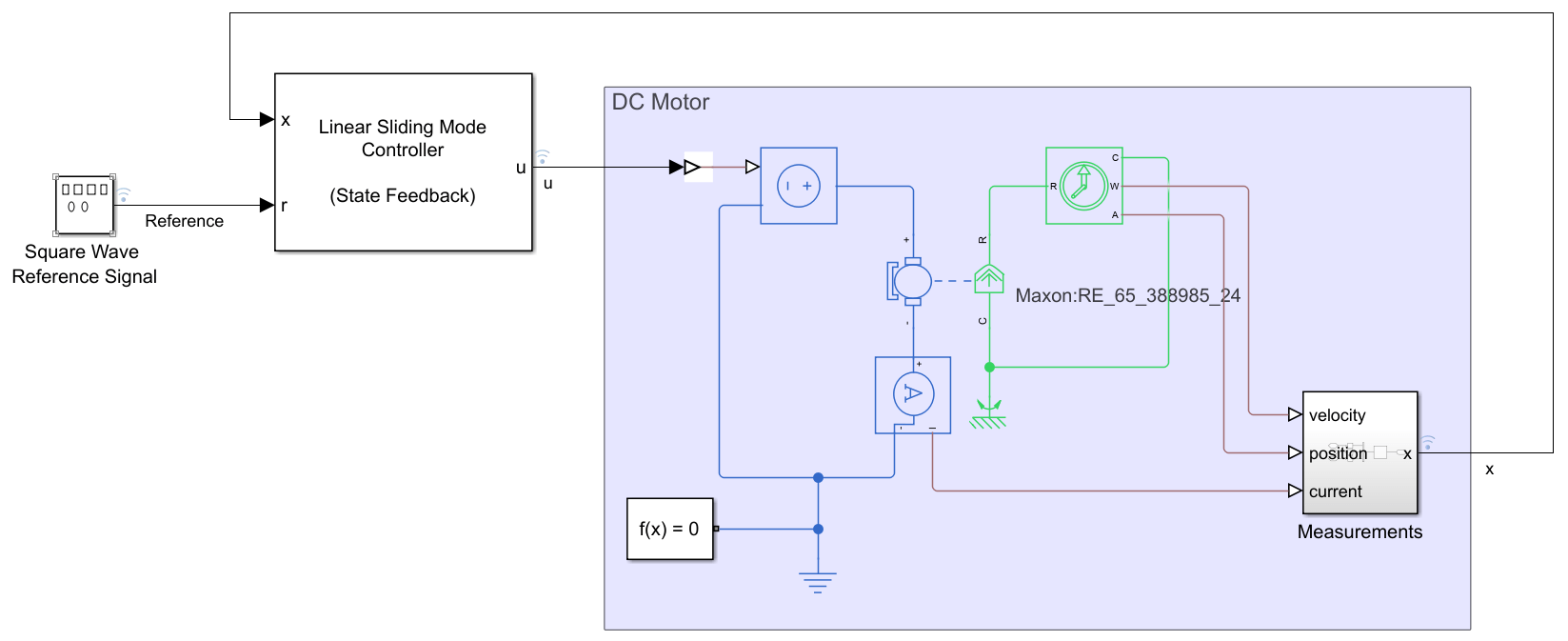

This example provides a model with a preconfigured Linear Sliding Mode Controller (State Feedback) block. To examine the configuration of the Linear Sliding Mode Controller (State Feedback) block, open the block parameters.

open_system('smc_dc_motor/Linear Sliding Mode Controller (State Feedback)')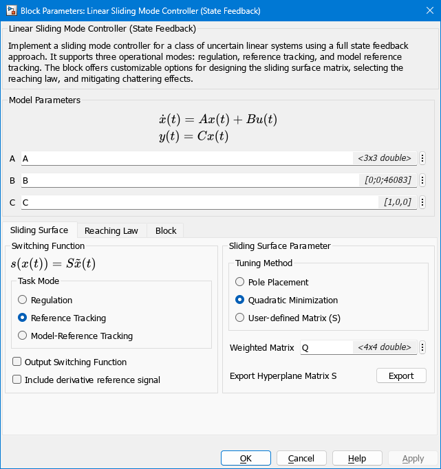

Simulate the system using the true values.

sim_nominal = sim('smc_dc_motor');

To illustrate real-world applications, where exact model parameters are not always known, simulate the system with perturbed values for the armature resistance and inductance. This helps demonstrate the robustness of the SMC approach.

% Perturbation in parameters
Ra=Ra*.7;
La=La*.7;

% Update system matrices
A = [0, 1, 0; 0, -v/J, Ki/J; 0, -Kv/La, -Ra/La];
B = [0; 0; 1/La];

% Simulate with perturbed parameters
sim_perturbed = sim('smc_dc_motor');

The simulation results, extracted and plotted, show the motor position and control input under both nominal and perturbed conditions.

nominal = sim_nominal.logsout.extractTimetable;
nominal = splitvars(nominal,'x','NewVariableNames',["Position", "Velocity", "Current"]);

perturbed = sim_perturbed.logsout.extractTimetable;
perturbed = splitvars(perturbed,'x','NewVariableNames',["Position", "Velocity", "Current"]);

stackedplot(nominal, perturbed,{["Position", "Reference"],"u"})

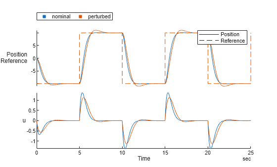
This example highlights the effectiveness of the sliding mode controller in tracking a reference signal, even when there are uncertainties in the system parameters. The robust nature of SMC makes it suitable for applications where parameter variations and external disturbances are present.