Stabilize Chua System Using Sliding Mode Controller

Since R2025a

This example show how to design a sliding mode controller (SMC) to stabilize a Chua system. Chua circuit is a well-known electronic circuit capable of exhibiting chaotic behavior, making it a fundamental component in chaos theory studies. The circuit consists of a nonlinear resistor (Chua diode), two capacitors, an inductor, and linear resistors, and was among the first circuits to generate chaotic signals.

Nonlinear Model

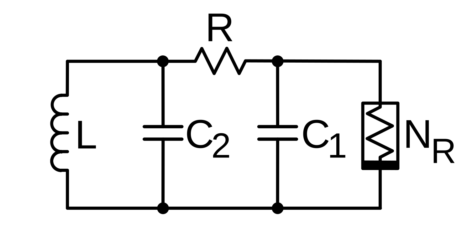
In this example, Chua diode is placed in parallel with capacitor ${\mathit{C}}_1$, introducing the nonlinearity essential for chaos. The circuit also includes a resistor and a series combination of capacitor ${\mathit{C}}_2$ and inductor $\mathit{L}$. These components interact to produce complex dynamics, with the voltages across ${\mathit{C}}_1$ and ${\mathit{C}}_2$ and the current through $\mathit{L}$ evolving over time. The system behavior is highly sensitive to its parameters, providing a rich platform for exploring chaotic phenomena. The dynamics of the circuit are described by the following equations:

$$\begin{array}{l}\frac{{\mathrm{dv}}_1}{\mathrm{dt}}=\frac{{\mathit{v}}_2-{\mathit{v}}_1}{{\mathit{RC}}_1}-\frac{\mathit{g}\left({\mathit{v}}_1\right)}{{\mathit{C}}_1}\\ \frac{{\mathrm{dv}}_2}{\mathrm{dt}}=\frac{{\mathit{v}}_1-{\mathit{v}}_2}{{\mathit{RC}}_2}+{\mathit{i}}_{\mathit{L}}\\ \frac{{\mathrm{di}}_{\mathit{L}}}{\mathrm{dt}}=-\frac{{\mathit{v}}_2}{\mathit{L}}+\mathit{u}\end{array}$$

Here, the constitutive relation of the nonlinear resistor is defined as $\mathit{g}\left({\mathit{v}}_1\right)=-\frac{1}{5}{\mathit{v}}_1\left(1-{\mathit{v}}_1^2\right)$

Define the model parameters.

R  = 1/0.7; % Resistance in Ohms (Ω)
L  = 1/7;   % Inductance of L in Henrys (H)
C1 = 1/10;  % Capacitance of C1 in Farad (F)
C2 = 1/0.5; % Capacitance of C2 in Farad (F)

Simulation

To observe the open loop behavior of the system, set the initial state variables and simulate the dynamics.

Define the initial state of the circuit.

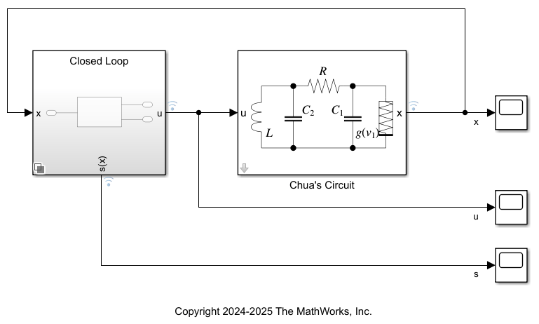
x0 = [0.4; 0.2; 0.5]; % [v1, v2, il]

Open the system and select the variant of the controller subsystem as OpenLoop.

open_system('smc_chua_system');
set_param('smc_chua_system/Variant Subsystem','OverrideUsingVariant','OpenLoop')

Simulate the model.

simOpenLoop = sim('smc_chua_system',100);

Plot the state responses onto $\left({\mathit{i}}_{\mathit{L}},{\mathit{V}}_1\right)$, $\left({\mathit{i}}_{\mathit{L}},{\mathit{V}}_2\right)$, and $\left({\mathit{V}}_1,{\mathit{V}}_2\right)$ planes.

plotResults('Open-Loop Simulation', simOpenLoop);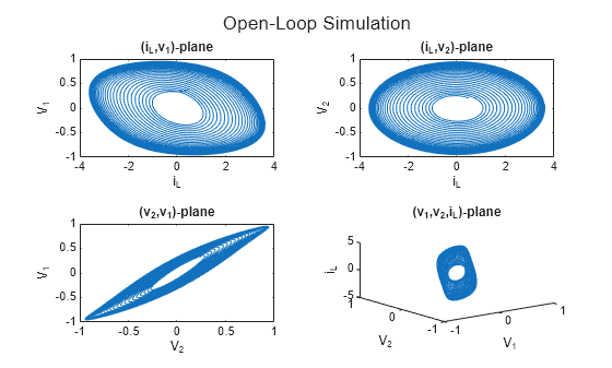

SMC Controller

To implement SMC, this example uses the Linear Sliding Mode Controller (State Feedback) block. This block requires model parameters in the form of matrices $\mathit{A}$ and$\mathit{B}$ for a regulation problem. Considering the Chua's diode as a bounded disturbance, you can rewrite the model dynamics using a state-space representation,$\dot{\mathit{x}}\left(\mathit{t}\right)=\mathit{Ax}\left(\mathit{t}\right)+\mathit{Bu}\left(\mathit{t}\right)+\mathit{d}\left(\mathit{x}\right)$.

The state vector is $\mathit{x}\left(\mathit{t}\right)={\left[\begin{array}{ccc}{\mathit{v}}_1& {\mathit{v}}_2& {\mathit{i}}_{\mathit{L}}\end{array}\right]}^{\mathit{T}}$and the state space representation is defined as:

$$\underset{}{\overset{\dot{}}{x}}(t)=\underset{A}{\underbrace{\stackrel{}{\left[\begin{array}{ccc}-\frac{1}{R{C}_1}& \frac{1}{R{C}_1}& 0\\ \frac{1}{R{C}_2}& \frac{1}{R{C}_2}& 1\\ 0& -\frac{1}{L}& 0\end{array}\right]}}}x(t)+\underset{B}{\underbrace{\stackrel{}{\left[\begin{array}{l}0\\ 0\\ 1\end{array}\right]}}}u(t)+\underset{d}{\underbrace{\stackrel{}{\left[\begin{array}{c}-\frac{g\left(x_1\right)}{C_1}\\ 0\\ 0\end{array}\right]}}}$$

Here, the term $\mathit{d}$ is considered as the disturbance for this example.

Define the matrices.

A = [-1/(C1*R), 1/(C1*R), 0; 1/(C2*R), -1/(C2*R), 1/C2; 0, -1/L, 0];
B = [0; 0; 1];

The model provided with this example is preconfigured to use the Linear Sliding Mode Controller block with the following parameter values:

• Reaching Rate (η) = 4

• Control Gain (κ) = 1

• Weighted Matrix = diag([10 10 1])

Note that the Reaching Rate (η) and Control Gain (κ) are parameters related to the reaching law, which dictates how quickly the system states converge to the sliding surface. The Weighted Matrix, on the other hand, characterizes the system dynamics once it is on the sliding surface, influencing the system response and stability during sliding mode operation. These parameters collectively shape the controller's performance in stabilizing the chaotic behavior of the Chua circuit.

To enable the Sliding Mode Controller, set the subsystem to ClosedLoop.

set_param('smc_chua_system/Variant Subsystem','OverrideUsingVariant','ClosedLoop')

Simulate the model without a boundary layer:

set_param(['smc_chua_system/Variant Subsystem/Closed Loop/' ...
    'Linear Sliding Mode Controller (State Feedback)'], 'BoundaryLayer', 'Sign');
simNoBoundaryLayer = sim('smc_chua_system',5);

Plot the open-loop and closed-loop simulation results.

plotResults('Open/Closed-Loop Simulation', simOpenLoop, simNoBoundaryLayer);

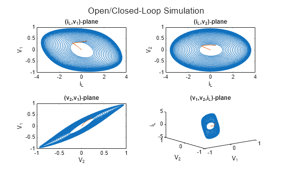
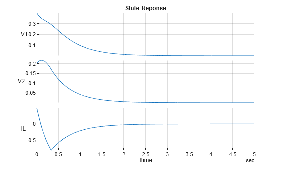
As illustrated in the plot, the sliding mode controller effectively drives the system state variables to zero from the initial conditions. This demonstrates the controller capability to stabilize the chaotic dynamics of the Chua circuit, ensuring that the states converge to the desired equilibrium point. The closed-loop response highlights the efficiency of the SMC in regulating the system behavior, contrasting with the open-loop scenario where the system exhibits chaotic characteristics.

Plot the state response.

figure;
simNoBoundaryLayer = simNoBoundaryLayer.logsout.extractTimetable;
simNoBoundaryLayer = splitvars(simNoBoundaryLayer,"x", "NewVariableNames",["V1", "V2", "iL"]);

s = stackedplot(simNoBoundaryLayer,["V1","V2","iL"]);
s.Title = 'State Reponse';
s.GridVisible = "on";

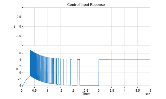
Plot the control input response.

s = stackedplot(simNoBoundaryLayer,["s","u"]);
s.Title = 'Control Input Reponse';
s.GridVisible = "on";

Reducing Chattering with Hyperbolic Tangent Boundary Layer

In sliding mode control, a common issue is the phenomenon known as chattering. Chattering is characterized by high-frequency oscillations in the control input, which can lead to undesirable effects such as increased wear in mechanical systems or noise in electronic circuits. To mitigate this, you can use a boundary layer approach.

This example uses a hyperbolic tangent function as the boundary layer to smooth the control action and reduce chattering. The hyperbolic tangent function provides a continuous transition around the sliding surface, effectively acting as a saturation function that limits the control effort within a specified range.

Set the controller to use the hyperbolic tangent boundary layer:

set_param('smc_chua_system/Variant Subsystem/Closed Loop/Linear Sliding Mode Controller (State Feedback)',...
    'BoundaryLayer', 'Hyperbolic Tangent');

Simulate the model with the boundary layer:

simWithBoundaryLayer = sim('smc_chua_system',5);

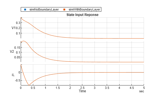
After applying the boundary layer, the control input becomes smoother, and the chattering effects are significantly reduced. You can observe this by comparing the control input and state responses with and without the boundary layer.

Plot the results to visualize the effect of the hyperbolic tangent boundary layer:

figure;
simWithBoundaryLayer = simWithBoundaryLayer.logsout.extractTimetable;
simWithBoundaryLayer = splitvars(simWithBoundaryLayer,"x", "NewVariableNames",["V1", "V2", "iL"]);

s = stackedplot(simNoBoundaryLayer, simWithBoundaryLayer,["V1","V2","iL"]);
s.Title = 'State Input Reponse';
s.GridVisible = "on";

s = stackedplot(simNoBoundaryLayer, simWithBoundaryLayer,"u");
s.Title = 'Control Input Reponse';
s.GridVisible = "on";

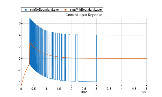
This example highlights the effectiveness of the sliding mode controller in regulating the states of Chua system to zero, considering the nonlinearity effect as a bounded disturbance in the controller design. Additionally, it underscores the use of a hyperbolic tangent boundary layer in sliding mode control, which effectively reduces chattering and leads to smoother control actions. This approach enhances the practical applicability of sliding mode controllers in real-world systems, where chattering can be detrimental to system performance and longevity.