Linear Sliding Mode Controller (State Feedback)

Design sliding mode control with knowledge of linear systems using state feedback

Since R2025a

• 

Libraries:
Simulink Control Design / Sliding Mode

Description

Use the Linear Sliding Mode Controller (State Feedback) block to implement Sliding Mode Control (SMC) based on a class of uncertain linear systems using a state feedback approach. This block offers the major benefit of providing two methods to automatically design the sliding surface based on a linear plant model. You can use the Sliding Mode Controller (Reaching Law) block to support a generic nonlinear plant model ($$\dot{x}=f(x)+g(x)u$$), though you need to design the sliding surface C yourself. In contrast, with the Linear Sliding Mode Controller (State Feedback) block, which is based on a nominal linear plant model, you can automatically design the sliding surface using the provided methods.

With this block, you can implement SMC in the following modes of operation:

• Regulation mode — Use this mode when you want to drive the system states x(t) to zero.

  $$\dot{x}(t)=Ax(t)+Bu(t)$$

• Reference tracking mode — Use this mode when you want the system output y(t) to follow a specified reference signal r(t).

  $$\begin{array}{l}\dot{x}(t)=Ax(t)+Bu(t)\\ y(t)=Cx(t)\end{array}$$

• Model reference tracking mode — Use this mode when you want the system states x(t) to track predefined reference model states x_m(t).

  $$\begin{array}{l}\dot{x}(t)=Ax(t)+Bu(t)\\ {\dot{x}}_m(t)=A_m{x}_m(t)+B_{m}r(t)\end{array}$$

For each mode, you can either specify the sliding matrix S explicitly or design the matrix using one of following two methods:

• Pole Placement — This method assigns the eigenvalues of the closed-loop system during the sliding mode to achieve the desired dynamic characteristics.

• Quadratic Minimization — This method designs the matrix S such that the system minimizes a quadratic performance index, expressed as:

  $$J=\frac{1}{2}{\displaystyle \underset{t_s}{\overset{\infty }{\int }}x{(t)}^{T}Qx(t)}dt$$

Additionally, you can choose a reaching law to control the rate of convergence to the sliding surface and a boundary layer to minimize chattering effects. For more information about SMC, see Sliding Mode Control.

Examples

New

Stabilize Chua System Using Sliding Mode Controller

Design sliding mode controller to stabilize a chaotic system.

• Since R2025a
• Open Live Script

New

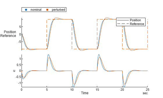
Sliding Mode Control of DC Motor

Design SMC for reference tracking for a DC motor.

• Since R2025a
• Open Live Script

Ports

Input

x — System states

scalar | vector

System states, specified as an n_x-by-1 signal, where n_x is the number of states.

Data Types: single | double

r — Reference signal

scalar | vector

Reference trajectory to follow in the tracking mode, specified as an n_y-by-1 signal, where n_y is the number of outputs.

The reference signal must be differentiable.

Dependencies

To enable this port, set Task Mode to Reference Tracking or Model-Reference Tracking.

Data Types: single | double

r.dot — Derivative of reference signal

scalar | vector

Derivative of the reference signal, specified as an n_y-by-1 signal, where n_y is the number of outputs.

Use this port when you want to provide the derivative of reference signal from an external input. Otherwise, the block computes the derivative during simulation.

Dependencies

To enable this port:

• Set Switching Function to Reference Tracking.

• Enable Include derivative reference signal.

Data Types: single | double

Output

u — Control action

scalar | vector

Computed control action, returned as an n_u-by-1 signal, where n_u is the number of inputs.

Data Types: single | double

s(x) — Switching function value

scalar | vector

Switching function value, returned as an n_u-by-1 signal, where n_u is the number of inputs.

Dependencies

To enable this port, enable the Output Switching Function parameter.

Data Types: single | double

Parameters

To edit block parameters interactively, use the Property Inspector. From the Simulink^® Toolstrip, on the Simulation tab, in the Prepare gallery, select Property Inspector.

Model Parameters

A — State matrix

[0 1; 0 0] (default) | square matrix

State matrix of the system, specified as a square matrix of size n_x-by-n_x, where n_x is the number of states. Here, the system is a class of uncertain linear systems with a nominal model defined by:

$$\dot{x}(t)=Ax(t)+Bu(t)$$

The pair (A,B) must be controllable.

Programmatic Use

To set the block parameter value programmatically, use the set_param function.

Parameter:	A
Values:	"[0 1; 0 0]" (default) | square matrix

Example: set_param(gcb,"A","[1 2; 3 1]")

B — Input matrix

[0; 1] (default) | matrix

Input matrix of the system, specified as a matrix of size n_x-by-n_u, where n_x is the number of states and n_u is the number of inputs. Here, the system is a class of uncertain linear systems with a nominal model defined by:

$$\dot{x}(t)=Ax(t)+Bu(t)$$

The pair (A,B) must be controllable.

Programmatic Use

To set the block parameter value programmatically, use the set_param function.

Parameter:	B
Values:	"[0; 1]" (default) | matrix

Example: set_param(gcb,"B","[2; 3]")

C — Output matrix

[1 0] (default) | matrix

Output matrix of the system, specified as a matrix of size n_y-by-n_x, where n_x is the number of states and n_y is the number of outputs. Here, the system is a class of uncertain linear systems with a nominal model defined by:

$$\begin{array}{l}\dot{x}(t)=Ax(t)+Bu(t)\\ y(t)=Cx(t)\end{array}$$

The system (A,B,C) must be completely controllable and have no invariant zeros at the origin.

Dependencies

To enable this parameter, set Task Mode to Reference Tracking.

Programmatic Use

To set the block parameter value programmatically, use the set_param function.

Parameter:	C
Values:	"[1 0]" (default) | matrix

Example: set_param(gcb,"C","[2 3]")

Reference Model Parameters

Am — Reference model state matrix

[0 1; 0 0] (default) | matrix

State matrix of the reference model, specified as a square matrix of size n_x-by-n_x, where n_x is the number of states. In the model-reference tracking mode, the specified system states x(t) track the reference model states x_m(t).

$$\begin{array}{l}\dot{x}(t)=Ax(t)+Bu(t)\\ {\dot{x}}_m(t)=A_m{x}_m(t)+B_{m}r(t)\end{array}$$

The pair (A_m,B_m) must be controllable and the reference model must be stable, that is, eigenvalues of A_m have negative real parts.

Dependencies

To enable this parameter, set Task Mode to Model-Reference Tracking.

Programmatic Use

To set the block parameter value programmatically, use the set_param function.

Parameter:	Am
Values:	"[0 1; 0 0]" (default) | square matrix

Example: set_param(gcb,"Am","[1 2; 3 1]")

Bm — Reference model input matrix

[0; 1] (default) | matrix

Input matrix of the reference model, specified as a square matrix of size n_x-by-n_u, where n_x is the number of states and n_u is the number of inputs. In the model-reference tracking mode, the specified system states x(t) track the reference model states x_m(t).

$$\begin{array}{l}\dot{x}(t)=Ax(t)+Bu(t)\\ {\dot{x}}_m(t)=A_m{x}_m(t)+B_{m}r(t)\end{array}$$

Dependencies

To enable this parameter, set Task Mode to Model-Reference Tracking.

Programmatic Use

To set the block parameter value programmatically, use the set_param function.

Parameter:	Bm
Values:	"[0; 1]" (default) | matrix

Example: set_param(gcb,"Bm","[2; 3]")

Sliding Surface Tab

Task Mode — Mode of operation

Regulation (default) | Reference Tracking | Model-Reference Tracking

Block mode of operation, specified as one of the following:

• Regulation — Use this mode when you want to drive the system states x(t) to zero.

  $$\dot{x}(t)=Ax(t)+Bu(t)$$

• Reference Tracking — Use this mode when you want the system output y(t) to follow a specified reference signal r(t).

  $$\begin{array}{l}\dot{x}(t)=Ax(t)+Bu(t)\\ y(t)=Cx(t)\end{array}$$

• Model-Reference Tracking — Use this mode when you want the system states x(t) to track predefined reference model states x_m(t).

  $$\begin{array}{l}\dot{x}(t)=Ax(t)+Bu(t)\\ {\dot{x}}_m(t)=A_m{x}_m(t)+B_{m}r(t)\end{array}$$

Programmatic Use

To set the block parameter value programmatically, use the set_param function.

Parameter:	TaskMode
Values:	"Regulation" (default) | "Reference Tracking" | "Model-Reference Tracking"

Example: set_param(gcb,"TaskMode","Reference Tracking")

Output Switching Function — Output switching function

off (default) | on

Select to return the sliding surface value at an output port s(x).

Programmatic Use

To set the block parameter value programmatically, use the set_param function.

Parameter:	EnableSwitchingFunction
Values:	"off" (default) | "on"

Example: set_param(gcb,"EnableSwitchingFunction","on")

Include derivative reference signal — Specify derivative of reference signal externally

off (default) | on

Select to specify the derivative of state reference signal externally at the input port r.dot.

Dependencies

To enable this parameter, set Task Mode to Reference Tracking.

Programmatic Use

To set the block parameter value programmatically, use the set_param function.

Parameter:	EnableTrackingDerivative
Values:	"off" (default) | "on"

Example: set_param(gcb,"EnableTrackingDerivative","on")

Sr — Design matrix for reference tracking

0.1 (default) | scalar | matrix

Design matrix to govern the reduced-order motion in the reference tracking mode, specified as a scalar or matrix of size n_y-by-n_y, where n_y is the number of outputs.

In reference tracking mode, the switching function is defined by:

$$\begin{array}{l}s(x)=S\tilde{x}(t)-S_{r}r(t)\\ \begin{array}{cc}\tilde{x}(t)=\left[\begin{array}{c}{x}_r(t)\\ x(t)\end{array}\right],& {\dot{x}}_r(t)=r(t)-y(t)\end{array}\end{array}$$

Dependencies

To enable this parameter, set: Task Mode to Reference Tracking and enable Include derivative reference signal.

Programmatic Use

To set the block parameter value programmatically, use the set_param function.

Parameter:	Sr
Values:	"0.1" (default) | scalar or matrix in quotes

Example: set_param(gcb,"Sr","eye(2)")

Tuning Method — Sliding surface design method

Pole Placement (default) | Quadratic Minimization | User-Defined Matrix (S)

Tuning method for designing sliding surface S, specified as one of the following:

• Pole Placement — This method assigns the eigenvalues of the closed-loop system during the sliding mode to achieve the desired dynamic characteristics. To specify the pole locations, use the Pole Location parameter.

• Quadratic Minimization — This method designs the matrix S such that the system minimizes a quadratic performance index, expressed as:

  $$J=\frac{1}{2}{\displaystyle \underset{t_s}{\overset{\infty }{\int }}x{(t)}^{T}Qx(t)}dt$$

  To specify the matrix Q, use the Weighted Matrix parameter.

• User-Defined Matrix (S) — Explicitly define the sliding surface matrix. To specify the matrix, use the block parameter S.

Programmatic Use

To set the block parameter value programmatically, use the set_param function.

Parameter:	Tuning
Values:	"Pole Placement" (default) | "Quadratic Minimization" | "User-defined Matrix (S)"

Example: set_param(gcb,"Tuning","Quadratic Minimization")

Pole Location — Pole location for pole placement method

-1 (default) | column vector

Pole location when designing sliding surface S using pole placement method, specified as a column vector of one of the following sizes:

• (n_x – n_u)-by-1 when Task Mode is set to either Regulation or Model-Reference Tracking.

• (n_x – n_u + n_y)-by-1 when Task Mode is set to Reference Tracking.

Dependencies

To enable this parameter, set Tuning Method to Pole Placement.

Programmatic Use

To set the block parameter value programmatically, use the set_param function.

Parameter:	PoleLocation
Values:	"-1" (default) | column vector in quotes

Example: set_param(gcb,"PoleLocation","[-2;-3]")

Weighted Matrix — Weighted matrix for quadratic performance index

eye(2) (default) | square matrix

Weighted matrix for quadratic performance index when designing sliding surface S using the quadratic minimization method, specified as a square matrix with one of the following sizes:

• n_x-by-n_x when Task Mode is set to either Regulation or Model-Reference Tracking.

• (n_x + n_y)-by-(n_x + n_y) when Task Mode is set to Reference Tracking.

Use the weighting matrix to penalize state deviations based on the assigned weight. This is the same notion as Q matrix in LQR design.

Dependencies

To enable this parameter, set Tuning Method to Quadratic Minimization.

Programmatic Use

To set the block parameter value programmatically, use the set_param function.

Parameter:	WeightedMatrix
Values:	"eye(2)" (default) | matrix in quotes

Example: set_param(gcb,"WeightedMatrix","[3 0; 0 1]")

Export Hyperplane Matrix S — Send designed hyperplane matrix to MATLAB^® workspace

button

When you click this button, the block creates a variable in the MATLAB workspace containing the designed hyperplane matrix S.

Dependencies

To enable this parameter, set Tuning Method to Pole Placement or Quadratic Minimization.

S — User-defined hyperplane matrix

[1 1] (default) | matrix

User-defined hyperplane matrix (S), specified as a matrix with one of the following sizes:

• n_u-by-n_x matrix when Task Mode is set to either Regulation or Model-Reference Tracking.

• n_u-by-(n_x + n_y) when Task Mode is set to Reference Tracking.

The matrix S determines the hyperplane to which the sliding mode control drives the system states.

Dependencies

To enable this parameter, set Tuning Method to User-defined Matrix (S).

Programmatic Use

To set the block parameter value programmatically, use the set_param function.

Parameter:	S
Values:	"[0; 1]" (default) | matrix

Example: set_param(gcb,"Bm","[2; 3]")

Reaching Law Tab

Reaching Law — Reaching law

Constant Rate (default) | Exponential | Power Rate | Unit Vector

Reaching law h(s(x)) for the sliding surface, specified as one of the following.

• Constant Rate — $$h\left(s\left(x\right)\right)=-{\eta }_i\theta \left(s_i\right)$$

  This law provides a constant rate to reach the sliding surface. Here, θ(s_i) is the boundary layer and η_i is the reaching rate of the ith control input.

• Exponential — $$h\left(s\left(x\right)\right)=-{\eta }_i\theta \left(s_i\right)-K_i{s}_i$$

  This law adds a term proportional to the sliding variable and provides a more aggressive convergence when the state deviation is significant. Here, K_i is the control gain term that scales the control effort associated with the ith sliding variable.

• Power Rate — $$h{\left(s\left(x\right)\right)}_i=-{\eta }_i{\left|s_i\right|}^{\alpha }\theta \left(s_i\right)$$

  This law provides fast reaching speed when the state is far away from the sliding surface, but reduces the speed as the state gets near. This ensures reduced chattering and provides fast convergence.

• Unit Vector — $$h\left(s\left(x\right)\right)=-\eta \theta \left(P_{2}s\right)-Ks$$

  Here, P₂ is the solution of the Lyapunov equation $$P_{2}K+K^T{P}_2=-I$$.

Programmatic Use

To set the block parameter value programmatically, use the set_param function.

Parameter:	ReachingLaw
Values:	"Constant Rate" (default) | "Exponential" | "Power Rate" | "Unit Vector"

Example: set_param(gcb,"ReachingLaw","Power Rate")

Reaching Rate (η) — Reaching rate

0.01 (default) | positive scalar | column vector

Reaching rate (η), specified as a positive scalar or a column vector of positive values with length equal to the number of control inputs.

Reaching rate determines the rate at which the system trajectory approaches the sliding surface. A larger value of η results in a faster convergence to the sliding surface but can also lead to higher control effort, which is not desirable in all cases due to potential issues like actuator saturation or increased chattering.

Programmatic Use

To set the block parameter value programmatically, use the set_param function.

Parameter:	ReachingRate
Values:	"0.01" (default) | positive scalar in quotes | column vector in quotes

Example: set_param(gcb,"ReachingRate","0.05")

Control Gain (K) — Control gain

0.01 (default) | positive scalar | column vector

Control gain of the proportional term in the exponential reaching law, specified as a positive scalar or column vector of length equal to the number of control inputs. In the exponential reaching law, this term increases the control effort proportional to the deviation from the sliding surface.

Dependencies

To enable this parameter, set Reaching Law to Exponential or Unit Vector.

Programmatic Use

To get the block parameter value programmatically, use the get_param function.

Parameter:	ControlGain
Values:	"0.01" (default) | positive scalar in quotes | column vector in quotes

Example: set_param(gcb,"ControlGain","2")

Power Rate Exponent (α) — Power rate exponent

0.01 (default) | positive scalar between 0 and 1 | column vector of positive values between 0 and 1

Exponent value in the power rate reaching law, specified as a positive scalar between 0 and 1 or column vector of length equal to the number of control inputs. This parameter determines the nonlinearity of the control action with respect to the distance from the sliding surface. Specifically, it adjusts how the control effort scales with the magnitude of the sliding variable. The value of α influences the smoothness of the approach to the sliding surface. The lower values lead to a softer approach and potentially reduce chattering.

Dependencies

To enable this parameter, set Reaching Law to Power Rate.

Programmatic Use

To set the block parameter value programmatically, use the set_param function.

Parameter:	PowerRate
Values:	"0.01" (default) | positive scalar between 0 and 1 in quotes | column vector of positive values between 0 and 1 in quotes

Example: set_param(gcb,"PowerRate","0.02")

Select Boundary Layer — Boundary layer function

Sign (default) | Relay | Hyperbolic Tangent | Saturation

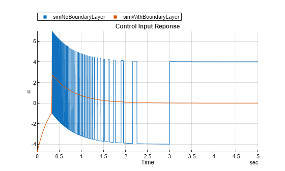
Boundary layer function, specified as one of the following:

• Sign — $$\theta \left(s\right)=sgn\left(s\left(x\right)\right)$$

  This option uses the default signum function and switches between –1 and 1 discontinuously.

• Relay — $$\theta \left(s\right)=\frac{s}{\left|s\right|+\varphi }$$

  This option uses a relay function to define the switching boundary around the sliding surface.

• Hyperbolic Tangent — $$\theta \left(s\right)=tanh\left(\frac{s}{\varphi }\right)$$

  This option uses a hyperbolic tangent function to define the switching boundary around the sliding surface.

• Saturation — $$\begin{array}{cc}\theta \left(s\right)=\{\begin{array}{c}\begin{array}{cc}1& s>\varphi \end{array}\\ \begin{array}{cc}ks& s\le \varphi \end{array}\\ \begin{array}{cc}-1& s<-\varphi \end{array}\end{array}& k=\frac{1}{\varphi }\end{array}$$

  This option uses a saturation function to smoothly interpolate between –1 and 1 when the sliding variable is within the boundary layer [–ϕ,ϕ], which reduces the high-frequency switching.

Programmatic Use

To set the block parameter value programmatically, use the set_param function.

Parameter:	BoundaryLayer
Values:	"Sign" (default) | "Relay" | "Hyperbolic Tangent" | "Saturation"

Example: set_param(gcb,""BoundaryLayer,"Saturation")

Phi — Boundary layer thickness

0.01 (default) | positive scalar | column vector

Boundary layer thickness parameter, specified as a positive scalar or column vector of length equal to the number of control inputs.

This parameter defines the boundary layer thickness around the sliding surface. A larger Phi value results in less chattering but can increase the steady-state error. Conversely, a smaller Phi value can reduce steady-state error but increase chattering.

Dependencies

To enable this parameter, set Select Boundary Layer to any one of these values:

• Relay

• Hyperbolic Tangent

• Saturation

Programmatic Use

To set the block parameter value programmatically, use the set_param function.

Parameter:	Phi
Values:	"0.01" (default) | positive scalar in quotes | column vector in quotes

Example: set_param(gcb,"Phi","0.05")

Enable zero-crossing detection — Enable zero-crossing detection

off (default) | on

Select to enable zero-crossing detection. For more information, see Zero-Crossing Detection.

Programmatic Use

To set the block parameter value programmatically, use the set_param function.

Parameter:	ZeroCross
Values:	"off" (default) | "on"

Example: set_param(gcb,"ZeroCross","on")

Block Tab

Time domain — Controller time domain

Continuous-Time (default) | Discrete-Time

Specify the controller time domain.

When you select Discrete-Time, specify the sample time using the Sample time parameter.

Programmatic Use

To set the block parameter value programmatically, use the set_param function.

Parameter:	TimeDomain
Values:	"Continous-Time" (default) | "Discrete-Time"

Example: set_param(gcb,""TimeDomain,"Discrete-Time")

Sample time — Sample time

-1 (default) | finite positive scalar

Sample time of the block, specified as a positive scalar. The block uses this value to sample the input-output data.

Dependencies

To enable this parameter, set the Time domain property to Discrete-Time.

Programmatic Use

To set the block parameter value programmatically, use the set_param function.

Parameter:	SampleTime
Values:	"-1" (default) | positive scalar in quotes

Example: set_param(gcb,"DiscreteTs","0.5")

Integrator method — Discrete-time integration method

Forward Euler (default) | Backward Euler | Trapezoidal

You can select one of the following integration methods for the discrete-time integrators.

• Forward Euler:

  $$y\left(n\right)=y\left(n-1\right)+T_s\cdot u\left(n-1\right)$$

• Backward Euler:

  $$y\left(n\right)=y\left(n-1\right)+T_s\cdot u\left(n\right)$$

• Trapezoidal:

  $$y\left(n\right)=y\left(n-1\right)+T_s\cdot \left[u\left(n\right)+u\left(n-1\right)\right]/2$$

Here:

• y is the integrator output

• u is the input

• n is the current sample time

• T_s is the sample time

For more information about discrete-time integration, see Discrete-Time Integrator.

Dependencies

To enable this parameter, set Time domain to Discrete-Time.

Programmatic Use

To set the block parameter value programmatically, use the set_param function.

Parameter:	IntegratorMethod
Values:	"Forward Euler" (default) | "Backward Euler" | "Trapezoidal"

Example: set_param(gcb,"IntegratorMethod","Trapezoidal")

Extended Capabilities

C/C++ Code Generation
Generate C and C++ code using Simulink® Coder™.

Version History

Introduced in R2025a