Main Content

zp2ctf

Convert zero-pole-gain filter parameters to cascaded transfer function form

Since R2024a

    Description

    [B,A] = zp2ctf(z,p) computes the second-order Cascaded Transfer Functions (CTF) of a filter system described by its zeros z and poles p.

    example

    [B,A] = zp2ctf(z,p,k) specifies the scalar gain of the system.

    example

    [B,A] = zp2ctf(___,Name=Value) specifies additional options using name-value arguments.

    example

    [___,gS] = zp2ctf(___) also returns the overall gain of the system.

    example

    Examples

    collapse all

    Compute the cascaded transfer function of a discrete-time system from its zeros and poles.

    z = [-1 -0.5+0.5i -0.5-0.5i];
    p = [0.77 0.9i -0.9i -0.3+0.4i -0.3-0.4i];
    
    [b,a] = zp2ctf(z,p)
    b = 3×3
    
             0    1.0000         0
             0    1.0000    1.0000
        1.0000    1.0000    0.5000
    
    
    a = 3×3
    
        1.0000   -0.7700         0
        1.0000    0.6000    0.2500
        1.0000         0    0.8100


    Convert a stopband filter represented with zeros, poles, and gain to cascaded transfer-function form.

    Get the zeros, poles, and gain of a 16th-order stopband Butterworth filter with stopband normalized frequencies of 0.35πrad/sample and 0.5πrad/sample.

    [z,p,k] = butter(16,[0.35 0.5],"stop");

    Compute the second-order cascaded transfer function coefficients. Plot the filter frequency response.

    [ctfB,ctfA] = zp2ctf(z,p,k);
    
    filterAnalyzer(ctfB,ctfA)

    Design a highpass filter and compute the zeros, poles, and gain. Convert a zero-pole-gain filter representation to cascaded transfer function. Customize the conversion with pole sorting and gain scaling options.

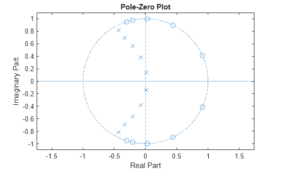
    Design a 10th-order type-II Chebyshev highpass filter sampled at 2000 Hz, with a cutoff frequency of 600 Hz and a stopband attenuation of 50 dB. Observe the z-plane showing five pairs of poles with a distance from the origin that ranges from 0 to 1.

    [z,p,k] = cheby2(10,50,600/(2000/2),"high");
    zplane(z,p,k)

    Figure contains an axes object. The axes object with title Pole-Zero Plot, xlabel Real Part, ylabel Imaginary Part contains 3 objects of type line. One or more of the lines displays its values using only markers

    Convert the zero-pole-gain filter representation to cascaded transfer function form. Sort the filter sections in descending order using the distance between the poles and the origin. Specify the gain scaling of the filter sections using the infinity norm. List the pole-origin distances for all the filter sections.

    [ctfBs,ctfAs] = zp2ctf(z,p,k,Direction="down",Scale="inf")
    ctfBs = 5×3
    
        0.6705    0.3993    0.6705
        0.6851    0.2758    0.6851
        0.5190   -0.0281    0.5190
        0.3424   -0.3002    0.3424
        0.2235   -0.4075    0.2235
    
    
    ctfAs = 5×3
    
        1.0000    0.8652    0.8531
        1.0000    0.6592    0.5958
        1.0000    0.4056    0.3591
        1.0000    0.1474    0.1505
        1.0000   -0.0262    0.0189
    
    
    % Pole-Origin Distances for all Filter Sections.
    numSections = size(ctfBs,1);
    poleRadius = zeros(numSections,2);
    for iter = 1:numSections
        poleRadius(iter,:) = abs(roots(ctfAs(iter,:))');
    end
    table((1:numSections)',poleRadius, ...
        VariableNames=["Section" "Pole-Origin Distances"])
    ans=5×2 table
        Section    Pole-Origin Distances
        _______    _____________________
    
           1        0.92363    0.92363  
           2        0.77188    0.77188  
           3        0.59926    0.59926  
           4        0.38792    0.38792  
           5        0.13735    0.13735  


    The cascade sections are sorted in descending order by pole-origin distance.

    Convert the zero-pole-gain representation of a Butterworth filter to cascaded transfer function form.

    Design a 6th-order Butterworth lowpass filter with a normalized cutoff frequency of 0.2πrad/sample.

    [z,p,k] = butter(6,0.2); 

    Obtain the numerator and denominator coefficients of the cascaded transfer function in the form of second-order and fourth-order cascaded transfer functions. Plot the frequency response of both cascaded transfer functions. Observe that both cascaded transfer functions yield the same frequency response.

    % Second-order
    [num2,den2,g2] = zp2ctf(z,p,k)
    num2 = 3×3
    
         1     2     1
         1     2     1
         1     2     1
    
    
    den2 = 3×3
    
        1.0000   -1.0321    0.2757
        1.0000   -1.1430    0.4128
        1.0000   -1.4044    0.7359
    
    
    g2 = 
    3.4054e-04
    
    % Fourth-order
    [num4,den4,g4] = zp2ctf(z,p,k,SectionOrder=4)
    num4 = 2×5
    
         1     2     1     0     0
         1     4     6     4     1
    
    
    den4 = 2×5
    
        1.0000   -1.0321    0.2757         0         0
        1.0000   -2.5474    2.7539   -1.4209    0.3038
    
    
    g4 = 
    3.4054e-04
    
    % Frequency response
    filterAnalyzer(num2,den2,num4,den4)

    Input Arguments

    collapse all

    System zeros and poles, specified as vectors.

    The vectors z and p contain the n zeros and m poles of the transfer function H(z), respectively.

    H(z)=k(zz1)(zz2)(zzn)(zp1)(zp2)(zpm).

    Example: zp2ctf([-1 -1],[0.5+0.5i 0.5-0.5i]) specifies [-1 -1] as zeros and [0.5+0.5i 0.5-0.5i] as poles.

    Data Types: single | double
    Complex Number Support: Yes

    System gain, specified as a real scalar.

    The scalar k represents the gain of the transfer function H(z).

    H(z)=k(zz1)(zz2)(zzn)(zp1)(zp2)(zpm).

    If you request the output argument gS, then the zp2ctf function assigns the value of k to gS.

    Data Types: single | double

    Name-Value Arguments

    Specify optional pairs of arguments as Name1=Value1,...,NameN=ValueN, where Name is the argument name and Value is the corresponding value. Name-value arguments must appear after other arguments, but the order of the pairs does not matter.

    Example: zp2ctf(-1,[0.6+0.4i 0.6-0.4i],Direction="down") converts a system with a zero in -1, poles in 0.6+0.4i and 0.6-0.4i, and a stacking order in descending distances between the poles and the origin of the z-plane.

    Order of the section transfer functions, specified as either 2 or 4. Depending on the value that you specify for SectionOrder, the zp2ctf function returns either the second-order or the fourth-order cascaded transfer function form.

    • 2 —The zp2ctf function returns second-order cascaded transfer function form matrices B and A with three columns each.

    • 4 —The zp2ctf function returns fourth-order cascaded transfer function form matrices B and A with five columns each.

    Data Types: single | double | int8 | int16 | int32 | int64 | uint8 | uint16 | uint32 | uint64

    Stacking order of the transfer function sections, specified as either "up" or "down". The zp2ctf function sorts the rows of A as a function of the distance between the poles and the origin, depending on the value you specify in Direction:

    • "up" — The first row of A contains the poles closest to the origin.

    • "down" — The first row of A contains the poles closest to the unit circle.

    The zp2ctf function sorts the rows of B so that the zeros in each section are paired with their closest poles associated with the rows of A.

    Data Types: char | string

    Gain scaling, specified as either "none", "inf", or "l2". The zp2ctf scales the gain and the numerator coefficients of all sections using the filternorm function, depending on the value you specify to "Scale":

    • "none" — No scaling

    • "inf" — Infinity-norm scaling

    • "l2" — L2-norm scaling

    Note

    • Infinity-norm and L2-norm scaling are appropriate only for direct-form II implementations, and they are supported only for stable systems.

    • Using infinity-norm scaling in conjunction with "up" directional ordering minimizes the probability of overflow when implementing the filter system. On the other hand, using L2-norm scaling in conjunction with "down" directional ordering minimizes the peak round-off noise.

    Data Types: char | string

    Output Arguments

    collapse all

    Cascaded transfer function coefficients, returned as either L-by-3 or L-by-5 matrices, where L is the number of sections. The number of columns depends on the value you specify in SectionOrder.

    The matrices B and A list the numerator and denominator coefficients of the cascaded transfer function, respectively. See Return Digital Filters in CTF Format for more information.

    Overall system gain, returned as a real-valued scalar.

    • If you specify to return gS, the zp2ctf function normalizes the numerator coefficients with respect to the system gain k and returns this gain in gS.

    • If you do not specify to return gS, the zp2ctf function uniformly distributes the system gain k across all system sections using the scaleFilterSections function.

    More About

    collapse all

    Cascaded Transfer Functions

    Partitioning an IIR digital filter into cascaded sections improves its numerical stability and reduces its susceptibility to coefficient quantization errors. The cascaded form of a transfer function H(z) in terms of the L transfer functions H1(z), H2(z), …, HL(z) is

    H(z)=l=1LHl(z)=H1(z)×H2(z)××HL(z).

    Return Digital Filters in CTF Format

    Specify B and A to return the filter coefficients. You can also specify gS to return the overall system gain of the filter. By specifying these output arguments, you can design digital filters in the CTF format for analysis, visualization, and signal filtering.

    Filter Coefficients

    When you specify to return the numerator and denominator coefficients in the CTF format, the L-row matrices B and A are returned as

    B=[b11b12b1,m+1b21b22b2,m+1bL1bL2bL,m+1],A=[1a12a1,n+11a22a2,n+11aL2aL,n+1],

    such that the full transfer function of the filter is

    H(z)=b11+b12z1++b1,m+1zm1+a12z1++a1,n+1zn×b21+b22z1++b2,m+1zm1+a22z1++a2,n+1zn××bL1+bL2z1++bL,m+1zm1+aL2z1++aL,n+1zn,

    where m ≥ 0 is the numerator order of the filter and n ≥ 0 is the denominator order.

    Note

    Coefficients and Gain

    You can specify to return the coefficients and overall system gain using the output argument triplet [B,A,gS]. In this case, the numerator coefficients are normalized, returning the filter coefficient matrices and gain as

    B=[1β12β1,m+11β22β2,m+11βL2βL,m+1],A=[1a12a1,n+11a22a2,n+11aL2aL,n+1],gS,

    so that the transfer function is

    H(z)=gS(1+β12z1++β1,m+1zm1+a12z1++a1,n+1zn×1+β22z1++β2,m+1zm1+a22z1++a2,n+1zn××1+βL2z1++βL,m+1zm1+aL2z1++aL,n+1zn).

    This transfer function is equivalent to the one defined in the Filter Coefficients section, where gS = b11×b21×...×bL1, and βli = bli/bl1 for i = 1,2,…,m and l = 1,2,…,L.

    Algorithms

    The zp2ctf function computes the numerator and denominator coefficients of the cascaded-transfer-function sections from the zeros, poles, and gain of the filter system. For an Nth-order filter system, there are (L!)2 possible combinations [1]. The variable L is the nearest integer greater than or equal to N/2 or N/4 for second-order or fourth-order sections, respectively.

    Customize the sorting criteria for pairing of the zeros and poles in the cascaded sections by specifying Direction to start with the poles and zeros closest to the origin of the z-plane ("up"), or closest to the unit circle ("down"). Perform gain scaling across the cascaded sections by specifying Scale. Customize the order of the cascaded sections by setting SectionOrder to either 2 or 4 to generate either second-order or fourth-order cascaded sections, respectively.

    The output arguments B and A contain the second-order or fourth-order cascaded transfer function coefficients of the filter system distributed in L rows.

    • Each row of A and B lists the coefficients in each section.

      • The function returns the first column of A as 1, thus A(1)=1 when A is a row vector.

      • If you specify to return gS, zp2ctf normalizes the numerator coefficients so that the first column of B is 1, and returns the overall system gain in gS. Thus, B(1)=1 when B is a row vector.

      • If you do not specify to return gS, zp2ctf first normalizes the numerator coefficients so that the first column of B is 1, and then uniformly multiplies sgn(gS)*gS^(1/L) to the normalized numerator coefficients, so that the first column of B is sgn(gS)*gS^(1/L). Thus, B(1)=gS when B is a row vector.

    • If you specify second-order sections or do not specify SectionOrder, the zp2ctf function returns the L-by-3 matrices B and A, where the last two columns correspond to the z–1 and z–2 terms for each cascaded section of the filter system.

    • If you specify fourth-order sections, the zp2ctf function returns the L-by-5 matrices B and A, where the last two columns correspond to the z–3 and z–4 terms for each cascaded section of the filter system.

    References

    [1] Lyons, Richard G. Understanding Digital Signal Processing. Upper Saddle River, NJ: Prentice Hall, 2004.

    Extended Capabilities

    C/C++ Code Generation
    Generate C and C++ code using MATLAB® Coder™.

    GPU Code Generation
    Generate CUDA® code for NVIDIA® GPUs using GPU Coder™.

    Version History

    Introduced in R2024a

    Go to top of page