Pool Dashboard

Monitor and visualize activity on parallel pools

Since R2025a

Description

Use the Pool Dashboard to collect and visualize monitoring data for interactive parallel pools.

Using this tool, you can:

• Collect monitoring data on how pool workers execute parallel constructs like parfor, parfeval, and spmd.

• Track the amount of data (in bytes) the client and workers send and receive.

• Understand the time each worker spends processing their portion of the parallel code.

• Examine communication patterns and identify bottlenecks and load-balancing issues.

Open the Pool Dashboard

• MATLAB^® Toolstrip: On the Home tab, in the Environment section, select Parallel > Open Pool Dashboard.

• Parallel status indicator: Click the indicator icon and select Open Pool Dashboard.

• MATLAB command prompt: Enter parpoolDashboard.

Examples

Investigate parfor-Loop with Pool Dashboard

This example shows how to use the Pool Dashboard to diagnose performance bottlenecks in parallel computations with parfor.

You have a computational task that calculates the maximum absolute eigenvalue of a 2-by-2 submatrix extracted from a large matrix. Initially, you implement this task using a for-loop. To accelerate the computation, you convert the for-loop into a parfor-loop, and run the parfor-loop on a pool with six workers. When you compare the execution times, the parfor-loop takes significantly longer than the serial for-loop. You can use the Pool Dashboard to investigate why the execution time for the parfor-loop is much larger than the serial for-loop.

Serial Execution	Parallel Execution
n = 10000; data = magic(n); out = zeros(n,1); tic for idx = 2:n thisData = idx*data(idx-1:idx,idx-1:idx); out(idx) = max(abs(eig(thisData))); end toc Elapsed time is 0.049732 seconds.	parpool("Processes",6) n = 10000; data = magic(n); out = zeros(n,1); tic parfor idx = 2:n thisData = idx*data(idx-1:idx,idx-1:idx); out(idx) = max(abs(eig(thisData))); end toc Elapsed time is 3.777290 seconds.

Open the Pool Dashboard.

To start collecting monitoring data, in the Monitoring section, select Start Monitoring. Start a parallel pool if you do not currently have an open parallel pool.

To collect monitoring data, in the MATLAB Command Window, run this code.

n = 10000;
data = magic(n);
out = zeros(n,1);
parfor idx = 2:n
    thisData = idx*data(idx-1:idx,idx-1:idx);
    out(idx) = max(abs(eig(thisData)));
end

Visualize the monitoring data. In the Monitoring section, select Update. The Pool Dashboard displays the monitoring results.

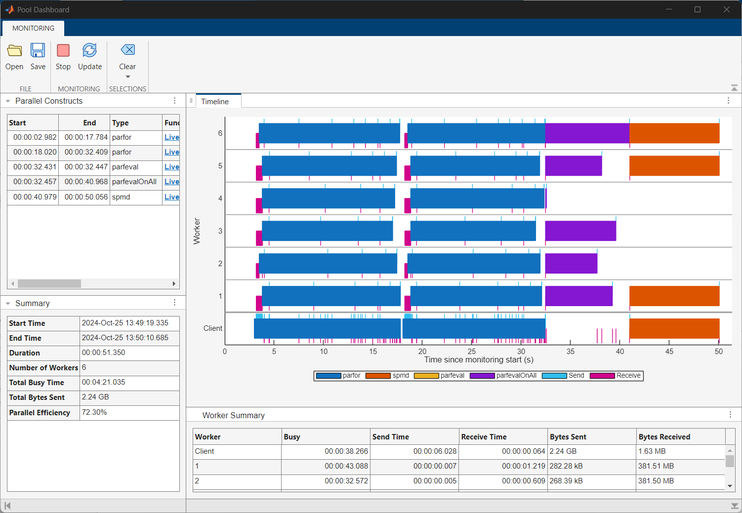
Review the monitoring data. The Timeline graph shows a visual representation of the time the workers and client spend running the parfor-loop and transferring data. Dark blue indicates time spent running the parfor-loop, light blue represents time spent sending data, and magenta represents time spent receiving data. You can observe that the workers spend the first two to three seconds of the computation receiving data from the client. Some workers also spend a considerable amount of time waiting to receive data from the client.

The Worker Summary table below the Timeline graph summarizes the information in the Timeline graph. To view the whole table, click the three dots on the right of the Worker Summary table and select Maximize.

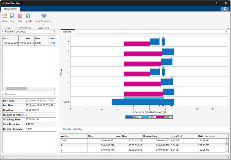
The workers spend a short time running the computations compared to transferring data. You can observe that the client sends a total of 4.47 GB of data to the workers and the workers each receive 762.95 MB of data while executing the parfor-loop. The parfor-loop requires all the workers to receive a copy of the input data, which introduces data transfer overheads to the computation that the for-loop does not have. The high parallel overhead dominates the computing time and this indicates the for-loop does not benefit from conversion into a parfor-loop.

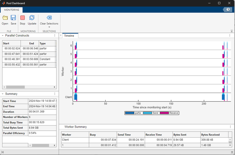
However, if you need to run a parfor-loop multiple times using the same set of data, you can optimize the parfor-loop by transferring the input data to the workers only once using a Constant object. This is a one off cost, and the workers have access to the data until you clear the Constant object.

To understand how using a Constant object optimizes the parfor-loop, run this code in the Command Window.

n = 10000;
data = magic(n);
out = zeros(n,1);

C = parallel.pool.Constant(data);

parfor idx = 1:10
    c = C.Value;
end

parfor idx = 2:n
    thisData = idx.*C.Value(idx-1:idx,idx-1:idx);
    out(idx) = max(abs(eig(thisData)));
end

Visualize the monitoring data. On the Monitoring tab, in the Monitoring section, select Update. The Pool Dashboard updates the displayed monitoring results.

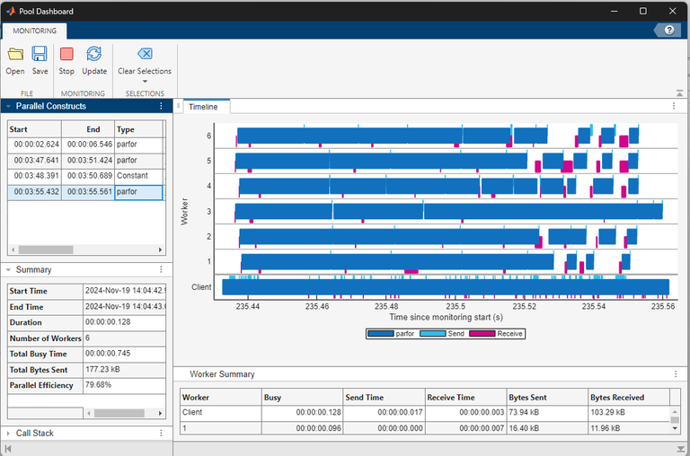
To view the monitoring data for only the parfor-loop that uses the Constant object, in the Parallel Constructs panel, select the last row in the table. When you use the Constant object to transfer data to the workers before you run the parfor-loop, the workers only spend time running the computations.

To stop collecting monitoring data, in the Monitoring section, select Stop.

Related Examples

• Monitor Pool Workers with Pool Dashboard
• Optimize parfor-Loops with Pool Dashboard

Programmatic Use

parpoolDashboard

parpoolDashboard opens the Pool Dashboard.

parpoolDashboard(monitoringResults)

parpoolDashboard(monitoringResults) opens the Pool Dashboard and displays the monitoring results in the ActivityMonitorResults object, monitoringResults.

Limitations

• Pool Dashboard is not supported on parallel pools of thread workers.

• Pool Dashboard is not supported on batch parallel pools. For a programmatic workflow, use an ActivityMonitor object instead. For details, see Programmatically Collect Pool Monitoring Data.

• The Timeline graph only displays information for a maximum of 32 workers.

Version History

Introduced in R2025a