addlink
Syntax
Description
linkIDs = addlink(graph,statePairs)navGraph
object.
linkIDs = addlink(graph,statePairs,metadata1,...metadataN)Weights, in addition to the state pairs.
However, the first column of the table must always specify the state pairs to be
connected.
Examples
Load navGraph object into MATLAB® workspace and inspect its properties.
load("navGraphData.mat")
disp(navGraphObj)
navGraph with properties:
States: [8×3 table]
Links: [7×3 table]
LinkWeightFcn: @nav.algs.distanceEuclidean
Inspect the states table of the graph.
disp(navGraphObj.States)
          StateVector          Name     Lanes
    _______________________    _____    _____

    8          2    0.72176    {'A'}      2
    1          1    0.29188    {'B'}      2
    7          7    0.91777    {'C'}      2
    8         10    0.71458    {'D'}      2
    5          1    0.54254    {'E'}      2
    3          6    0.14217    {'F'}      2
    2          9    0.37334    {'G'}      3
    8          7    0.67413    {'H'}      2
Inspect the links table of the graph. The first column contains the indices of states from the states table. The two-element vectors in the first column of the table represent the pairs of states that are connected. Note that the links table also contains 'Weight' and 'Curvature' metadata in addition to the connected state pairs.
disp(navGraphObj.Links)
    EndStates    Weight    Curvature
    _________    ______    _________

     1    3      1.5089    0.0034635
     3    7       8.921    0.0063649
     5    4       2.387    0.0060558
     6    2      19.452    0.0041751
     7    1      38.776    0.0051347
     7    8      13.938    0.0076324
     8    2      43.893    0.0031493
Display the graph.
show(navGraphObj)

From the graph, you can infer that the states 'D' and 'E' are not connected to any other states, and no path exists when a start or goal point lies on one of these states. To connect these states, use the addlink function. Specify the state pairs to be connected using either the indices or state names from the states table.
Specify State Indices to Add Links
From the states table of the input graph you can find that the indices for the states with names "E" and "F" are 5 and 6, respectively. Specify these indices as input to connect states "E" and "F".
Id = addlink(navGraphObj,[5 6],2.5,0.001)
Id =
4
Inspect the updated links table for new states and the related metadata. Note that the state indices of the new state pairs are added to the fifth row of the links table. The entries in the links table are sorted according to the index of the first state in each state pair listed in the first column. The rows that have the same index for the first state are sorted based on the index of the second state in each state pair.
disp(navGraphObj.Links)
    EndStates    Weight    Curvature
    _________    ______    _________

     1    3      1.5089    0.0034635
     3    7       8.921    0.0063649
     5    4       2.387    0.0060558
     5    6         2.5        0.001
     6    2      19.452    0.0041751
     7    1      38.776    0.0051347
     7    8      13.938    0.0076324
     8    2      43.893    0.0031493
Display the updated graph. Now all the states in the input graph are connected, you can compute path for any start and goal point that lie between these states.
show(navGraphObj)

Specify State Names to Add Links
Add a link between states with names "C" and "D". In addition to the state pair, you must also specify the value for associated Weight and Curvature metadata in the links table.
Id = addlink(navGraphObj,["C" "D"],5,0.004)
Id =
2
Inspect the updated links table for new state pairs and the related metadata. Note that the state indices of the new state pairs are added to the second row of the links table.
disp(navGraphObj.Links)
    EndStates    Weight    Curvature
    _________    ______    _________

     1    3      1.5089    0.0034635
     3    4           5        0.004
     3    7       8.921    0.0063649
     5    4       2.387    0.0060558
     5    6         2.5        0.001
     6    2      19.452    0.0041751
     7    1      38.776    0.0051347
     7    8      13.938    0.0076324
     8    2      43.893    0.0031493
show(navGraphObj)

Load navGraph object into MATLAB® workspace and inspect its properties.
load("navGraphData.mat")
disp(navGraphObj)
navGraph with properties:
States: [8×3 table]
Links: [7×3 table]
LinkWeightFcn: @nav.algs.distanceEuclidean
Inspect the states table of the graph.
disp(navGraphObj.States)
          StateVector          Name     Lanes
    _______________________    _____    _____

    8          2    0.72176    {'A'}      2
    1          1    0.29188    {'B'}      2
    7          7    0.91777    {'C'}      2
    8         10    0.71458    {'D'}      2
    5          1    0.54254    {'E'}      2
    3          6    0.14217    {'F'}      2
    2          9    0.37334    {'G'}      3
    8          7    0.67413    {'H'}      2
Inspect the links table of the graph. The first column contains the indices of states from the states table. The two-element vectors in the first column of the table represent the pairs of states that are connected. Note that the links table also contains 'Weight' and 'Curvature' metadata in addition to the connected state pairs.
disp(navGraphObj.Links)
    EndStates    Weight    Curvature
    _________    ______    _________

     1    3      1.5089    0.0034635
     3    7       8.921    0.0063649
     5    4       2.387    0.0060558
     6    2      19.452    0.0041751
     7    1      38.776    0.0051347
     7    8      13.938    0.0076324
     8    2      43.893    0.0031493
Display the graph. From the graph, you can infer that the states 'D' and 'E' are not connected to any other states, and no path exists when a start or goal point lies on one of these states.
show(navGraphObj)

Add links between these state pairs:
States with names "
C" and "D".States with names "
E" and "F".States with names "
H" and "D"
In addition to the state pairs, you must also specify the values for associated Weight and Curvature metadata in the links table. The function returns the indices of the new state pairs in the links table.
Id = addlink(navGraphObj,["C" "D";"E" "F";"H" "D"],[5;2.5;50],[0.005;0.003;0.004])
Id = 3×1

     2
     5
    10
Inspect the updated links table for new state pairs and their associated metadata. Note that the state indices of the new state pairs are added to the second, fifth, and tenth rows of the links table. The entries in the links table are sorted according to the index of the first state in each state pair listed in the first column. The rows that have the same index for the first state are sorted based on the index of the second state in each state pair.
disp(navGraphObj.Links)
    EndStates    Weight    Curvature
    _________    ______    _________

     1    3      1.5089    0.0034635
     3    4           5        0.005
     3    7       8.921    0.0063649
     5    4       2.387    0.0060558
     5    6         2.5        0.003
     6    2      19.452    0.0041751
     7    1      38.776    0.0051347
     7    8      13.938    0.0076324
     8    2      43.893    0.0031493
     8    4          50        0.004
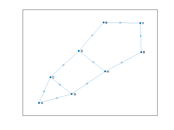
Display the updated graph.
show(navGraphObj)
Input Arguments
Output Arguments
Extended Capabilities
Version History
Introduced in R2024aSee Also
addstate | rmstate | rmlink | findlink | findstate | index2state | state2index | successors | show | copy