compare
Compare identified model output with measured output
Syntax
Description
Plot Simulated and Measured Outputs
compare(
simulates the response of a single dynamic system model data,sys)sys or an
array of dynamic system models, and superimposes the response for each model over the
plotted input/output measurement data contained in data.
data can be a timetable, a comma-separated input/output matrix
pair, or a data object such as an iddata object or an idfrd object.
The plot also displays the normalized root mean square (NRMSE) measure of the goodness of the fit between the simulated response and the output measurement data.
Use this function when you want to validate a single model or when you want to evaluate a set of candidate models identified from the same measurement data.
For timetables and data objects, compare matches the input/output
channels based on the channel names in sys and ignores nonmatching
channels.
compare( compares the
responses of multiple dynamic systems on the same axes. data,sys1,...,sysN)compare
automatically chooses the line specifications.
Predict Model Output
compare(___, predicts the
response of kstep)sys, using a prediction horizon specified by
kstep. Prediction uses output measurements as well as input
measurements to project a future response. kstep represents the
number of time samples between the timepoint of each output measurement and the timepoint
of the resulting predicted response.
For more information on prediction, see Simulate and Predict Identified Model Output. You can use this syntax with any of the previous input/output combinations.
Specify Additional Options
Examples
Identify a linear model and visualize the simulated model response with the data from which it was generated.
Load the input/output measurements in tt1, and identify a third-order state-space model sys.
load sdata1 tt1;
sys = ssest(tt1,3);
sys is a continuous-time identified state-space (idss) model.
Use compare to simulate the sys response and plot it alongside the data in tt1.
figure
compare(tt1,sys)
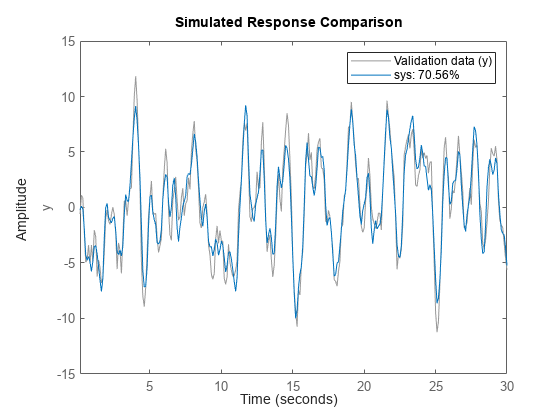
The plot illustrates the differences between the model response and the original data. The percentage shown in the legend is the NRMSE fitness value. It represents how close the predicted model output is to the data.
To change display options in the plot, right-click the plot to access the context menu. For example:
To plot the error between the predicted output and measured output, select Error Plot.
To view the confidence region for the simulated response, select Characteristics -> ConfidenceRegion.
To specify number of standard deviations to plot, double-click the plot and open the Property Editor dialog box. In the Options tab, specify the number of standard deviations in Confidence Region for Identified Models. The default value is
1standard deviation.
Identify a linear model and visualize the predicted model response with the data from which it was computed.
Identify a third-order state-space model using the input/output measurements in umat1 and ymat1.
load sdata1 umat1 ymat1 Ts
sys = ssest(umat1,ymat1,3,'Ts',Ts);
sys is a discrete-time identified state-space (idss) model.
Now use compare to plot the predicted response. Prediction differs from simulation in that it uses both measured input and measured output when computing the system response. The prediction horizon defines how far in the future to predict, relative to your current measured output point. For this example, set the prediction horizon kstep to 10 steps, and use compare to plot the predicted response against the original measurement data.
kstep = 10;
compare(umat1,ymat1,sys,kstep)
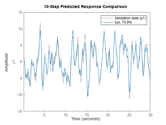
In this plot, each sys data point represents the predicted output associated with output measurement data that was taken at least 10 steps earlier. For instance, the point at t = 15s is based on output measurements taken at or prior to t = 5s. The calculation of this t = 15s sys data point also uses input measurements up to t = 15s, just as a simulation would.
The plot illustrates the differences between the model response and the original data. The percentage shown in the legend is the NRMSE fitness value. It represents how closely the predicted model output matches the data.
To change display and simulation options in the plot, right-click the plot to access the context menu. For example, to plot the error between the predicted output and measured output, select Error Plot from the context menu. To change the prediction horizon value, or to toggle between simulation and prediction, select Prediction Horizon from the context menu.
Identify several model types for the same data, and compare the results to see which best fits the data.
Load the data, which contains iddata object z1 with single input and output.
load iddata1;From z1, identify a model for each of the following linear forms:
ARMAX (
idpoly) of orders 2, 3, and 1, with dead time of 0State space (
idss) with three statesTransfer function (
idtf) with three poles
sys_armax = armax(z1,[2 3 1 0]);
sys_ss = ssest(z1,3);
sys_tf = tfest(z1,3);
Using compare, plot the simulated responses for the three models with z1.
compare(z1,sys_armax,sys_ss,sys_tf)
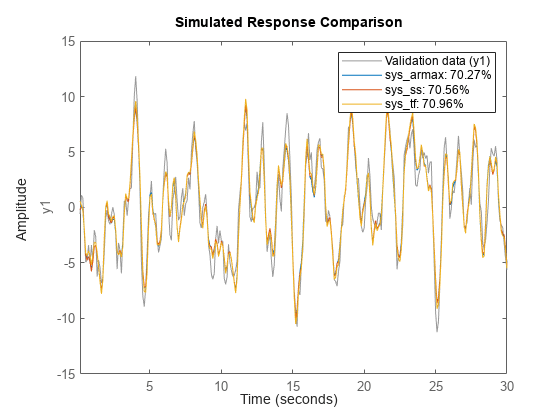
For this set of data, along with the default settings for all the models, the transfer-function form has the best NRMSE fit. However, the fits for all models are within about 1% of each other.
You can interactively control which model responses are displayed in the plot by right-clicking on the plot and hovering over Systems.
Compare the outputs of multiple estimated models of differing types to measured frequency-domain data.
For this example, estimate a process model and an output-error polynomial from frequency response data.
load demofr  % frequency response data
zfr = AMP.*exp(1i*PHA*pi/180);
Ts = 0.1;
data = idfrd(zfr,W,Ts);
sys1 = procest(data,'P2UDZ');
sys2 = oe(data,[2 2 1]);
sys1, an idproc model, is a continuous-time process model. sys2, an idpoly model, is a discrete-time output-error model.
Compare the frequency response of the estimated models to data.
compare(data,sys1,'g',sys2,'r');

The two models have NRMSE fit values that are nearly equal with respect to the data from which they were calculated.
Modify default behavior when you compare an estimated model to measured data.
Estimate a transfer function for measured data.
load sdata1 tt1;
sys = tfest(tt1,3);
sys is a continuous-time identified transfer function (idtf) model.
Suppose you want your initial conditions to be zero. The default for compare is to estimate initial conditions from the data.
Create an option set to specify the initial condition handling. To use zero for initial conditions, specify 'z' for the 'InitialCondition' option.
opt = compareOptions('InitialCondition','z');
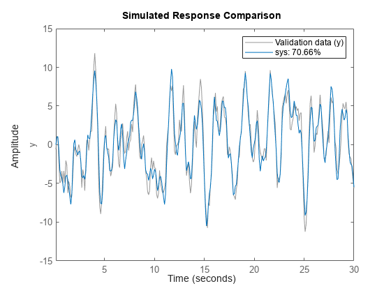
Compare the estimated transfer function model output to the measured data using the comparison option set.
compare(tt1,sys,opt)
Load the data.
load iddata2 z2
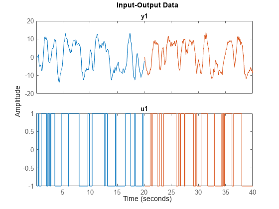
Split the data into estimation and validation sets.
z2e = z2(1:200);
z2v = z2(201:400);
idplot(z2e,z2v)
Estimate a state-space model and a transfer function model using the estimation data.
sys_ss = ssest(z2e,2);
sys_tf = tfest(z2e,2,1);
Use compare to obtain initial conditions ic_ss for sys_ss.
[y_ss,fit_ss,ic_ss] = compare(z2e,sys_ss);
ic_ss
ic_ss = 2×1

   -0.0018
    0.0016
ic_ss is a numeric vector of initial states.
Use compare to obtain initial conditions ic_tf for sys_tf.
[y_tf,fit_tf,ic_tf] = compare(z2e,sys_tf);
ic_tf
ic_tf =
  initialCondition with properties:

     A: [2×2 double]
    X0: [2×1 double]
     C: [-1.6093 5.1442]
    Ts: 0
ic_tf is an initialCondition object that contains, in state-space form, a model of the free response of sys_tf to the initial conditions. A and C contain the free-response information and X0 contains the initial states.
Now obtain initial conditions for both models at once using the validation data.
[y_sstf,fit_sstf,ic_sstf] = compare(z2v,sys_ss,sys_tf);
ic_sstf
ic_sstf=2×1 cell array
    {2×1 double          }
    {1×1 initialCondition}
ic_sstf is a cell array that contains an initial state vector for sys_ss and an initialCondition object for sys_tf.
compare can provide initial conditions for an existing model with any measurement data set.
Input Arguments
Output Arguments
Tips
The NRMSE fit result you obtain with
comparemay not precisely match the fit value reported in model identification. These differences typically arise from mismatches in initial conditions, and in the differences in the prediction horizon defaults for identification and for validation. The differences are generally small, and should not impact your model selection and validation workflow. For more information, see Resolve Fit Value Differences Between Model Identification and compare Command.comparematches the input/output channels indataandsysbased on the channel names. Thus, it is possible to evaluate models that do not use all the input channels that are available indata. This flexibility allows you to compare multiple models which were each identified independently from different sets of input/output channels.The
compareplot allows you to vary key parameters. For example, you can interactively control:Whether you generate a simulated or predicted response
Prediction horizon value
Initial condition handling
Which experiment data you view
Which system models you view
To access the controls, right-click the plot to bring up the options menu.
Version History
Introduced in R2006aSee Also
compareOptions | sim | predict | forecast | goodnessOfFit | chgTimeUnit | chgFreqUnit | idplot