Constrained Minimization Using ga, Problem-Based
This example shows how to minimize an objective function, subject to nonlinear inequality constraints and bounds, using ga in the problem-based approach. For a solver-based version of this problem, see Constrained Minimization Using the Genetic Algorithm.
Constrained Minimization Problem
For this problem, the fitness function to minimize is a simple function of 2-D variables X and Y.
camxy = @(X,Y)(4 - 2.1.*X.^2 + X.^4./3).*X.^2 + X.*Y + (-4 + 4.*Y.^2).*Y.^2;
This function is described in Dixon and Szego [1].
Additionally, the problem has nonlinear constraints and bounds.
   x*y + x - y + 1.5 <= 0  (nonlinear constraint)
   10 - x*y <= 0           (nonlinear constraint)
   0 <= x <= 1             (bound)
   0 <= y <= 13            (bound)
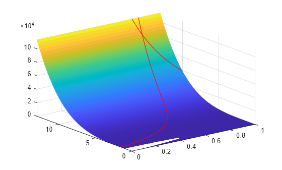
Plot the nonlinear constraint region on a surface plot of the fitness function. The constraints limit the solution to the small region above both red curves.
x1 = linspace(0,1);
y1 = (-x1 - 1.5)./(x1 - 1);
y2 = 10./x1;
[X,Y] = meshgrid(x1,linspace(0,13));
Z = camxy(X,Y);
surf(X,Y,Z,LineStyle="none")
hold on
z1 = camxy(x1,y1);
z2 = camxy(x1,y2);
plot3(x1,y1,z1,"r-",x1,y2,z2,"r-")
xlim([0 1])
ylim([0 13])
zlim([0,max(Z,[],"all")])
hold off
Create Optimization Variables, Problem, and Constraints
To set up this problem, create optimization variables x and y. Set the bounds when you create the variables.
x = optimvar("x",LowerBound=0,UpperBound=1);
y = optimvar("y",LowerBound=0,UpperBound=13);
Create the objective as an optimization expression.
cam = camxy(x,y);
Create an optimization problem with this objective function.
prob = optimproblem(Objective=cam);
Create the two nonlinear inequality constraints, and include them in the problem.
prob.Constraints.cons1 = x*y + x - y + 1.5 <= 0;
prob.Constraints.cons2 = 10 - x*y <= 0;
Review the problem.
show(prob)
  OptimizationProblem :

	Solve for:
       x, y

	minimize :
       (((((4 - (2.1 .* x.^2)) + (x.^4 ./ 3)) .* x.^2) + (x .* y)) + (((-4) + (4 .* y.^2)) .* y.^2))


	subject to cons1:
       ((((x .* y) + x) - y) + 1.5) <= 0

	subject to cons2:
       (10 - (x .* y)) <= 0

	variable bounds:
       0 <= x <= 1

       0 <= y <= 13
Solve Problem
Solve the problem, specifying the ga solver.
[sol,fval] = solve(prob,Solver="ga")Solving problem using ga. Optimization finished: average change in the fitness value less than options.FunctionTolerance and constraint violation is less than options.ConstraintTolerance.
sol = struct with fields:
    x: 0.8122
    y: 12.3103
fval =
9.1268e+04
Add Visualization
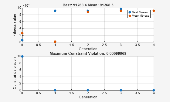
To observe the solver's progress, specify options that select two plot functions. The plot function gaplotbestf plots the best objective function value at every iteration, and the plot function gaplotmaxconstr plots the maximum constraint violation at every iteration. Set these two plot functions in a cell array. Also, display information about the solver's progress in the Command Window by setting the Display option to "iter".
options = optimoptions(@ga,...
    PlotFcn={@gaplotbestf,@gaplotmaxconstr},...
    Display="iter");
Run the solver, including the options argument.
[sol,fval] = solve(prob,Solver="ga",Options=options)Solving problem using ga.
Single objective optimization:
2 Variables
2 Nonlinear inequality constraints
Options:
CreationFcn: @gacreationuniform
CrossoverFcn: @crossoverscattered
SelectionFcn: @selectionstochunif
MutationFcn: @mutationadaptfeasible
Best Max Stall
Generation Func-count f(x) Constraint Generations
1 2520 91357.8 0 0
2 4982 91324.1 4.55e-05 0
3 7914 97166.6 0 0
4 16145 91268.4 0.0009997 0
Optimization finished: average change in the fitness value less than options.FunctionTolerance and constraint violation is less than options.ConstraintTolerance.
sol = struct with fields:
    x: 0.8123
    y: 12.3103
fval =
9.1268e+04
Nonlinear constraints cause ga to solve many subproblems at each iteration. As shown in both the plots and the iterative display, the solution process has few iterations. However, the Func-count column in the iterative display shows many function evaluations per iteration.
Unsupported Functions
If your objective or nonlinear constraint functions are not supported (see Supported Operations for Optimization Variables and Expressions), use fcn2optimexpr to convert them to a form suitable for the problem-based approach. For example, suppose that instead of the constraint , you have the constraint , where is the modified Bessel function besseli(1,x). (The Bessel functions are not supported functions.) Create this constraint using fcn2optimexpr. First, create an optimization expression for .
bfun = fcn2optimexpr(@(t,u)besseli(1,t) + besseli(1,u),x,y);
Next, replace the constraint cons2 with the constraint bfun >= 10.
prob.Constraints.cons2 = bfun >= 10;
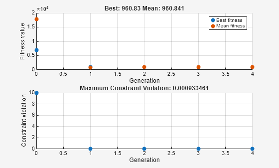
Solve the problem. The solution is different because the constraint region is different.
[sol2,fval2] = solve(prob,Solver="ga",Options=options)Solving problem using ga.
Single objective optimization:
2 Variables
2 Nonlinear inequality constraints
Options:
CreationFcn: @gacreationuniform
CrossoverFcn: @crossoverscattered
SelectionFcn: @selectionstochunif
MutationFcn: @mutationadaptfeasible
Best Max Stall
Generation Func-count f(x) Constraint Generations
1 2512 974.044 0 0
2 4974 960.998 0 0
3 7436 963.12 0 0
4 12001 960.83 0.0009335 0
Optimization finished: average change in the fitness value less than options.FunctionTolerance and constraint violation is less than options.ConstraintTolerance.
sol2 = struct with fields:
    x: 0.4999
    y: 3.9979
fval2 =
960.8300
References
[1] Dixon, L. C. W., and G .P. Szego (eds.). Towards Global Optimisation 2. North-Holland: Elsevier Science Ltd., Amsterdam, 1978.
See Also
ga | solve | fcn2optimexpr