Price Weather Derivatives
This example demonstrates a workflow for pricing weather derivatives based on historically observed temperature data.
The workflow for pricing call and put options for weather derivatives includes these steps:
The techniques used in this example are based on the approach described in Alaton [1].
What Is a Weather Derivative?
A weather derivative is a financial instrument used by companies or individuals to hedge against the risk of weather-related losses. Weather derivatives are index-based instruments that use observed weather data at a weather station to create an index on which a payout is based. The seller of a weather derivative agrees to bear the risk of disasters in return for a premium. If no damages occur before the expiration of the contract, the seller makes a profit—and in the event of unexpected or adverse weather, the buyer of the derivative claims the agreed amount.
How to Price Weather Derivatives
A number of different contracts for weather derivatives are traded on the over-the-counter (OTC) market. This example explores a simple option (call or put) based on the accumulation of heating degree days (HDD), which are the number of degrees that the temperature deviates from a reference level on a given day.
There is no standard model for valuing weather derivatives similar to the Black-Scholes formula for pricing European equity options and similar derivatives. The underlying asset of the weather derivative is not tradeable, which violates a number of key assumptions of the Black-Scholes model. In this example, you price the option using the following formula from Alaton [1]:
In general, the process of pricing weather derivative options is: obtain temperature data, clean the temperature data, and model the temperature to forecast the option price.
Get Raw Temperature Data
All data in this example is obtained from NOAA. Use getGHCNData in Local Functions to extract the data, given a stationID and start and end dates. A REST API is also available for extracting data from NOAA. For more information on using a REST API, see Pricing weather derivatives GitHub.
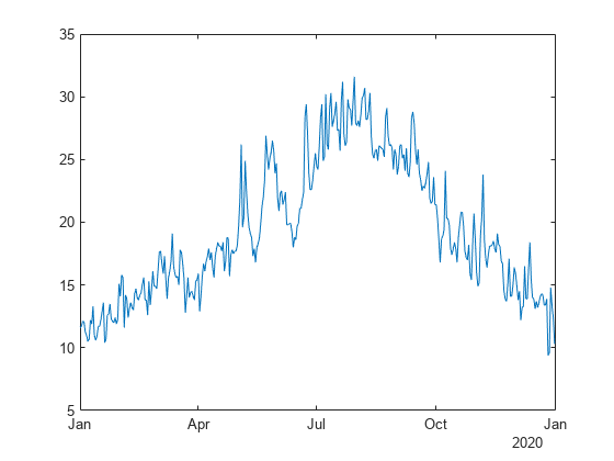
To obtain the full temperature data for one year and plot the results, use getGHCNData in Local Functions.
stationID = 'SPE00119783';
Element = 'TAVG';
startDate = datetime(2020,1,1);
endDate = datetime(2020,12,31);
T = getGHCNData(stationID,Element,startDate,endDate,false);
head(T)
       Date        TAVG
    ___________    ____

    01-Jan-2020    11.6
    02-Jan-2020    11.7
    03-Jan-2020    12.1
    04-Jan-2020    12.1
    05-Jan-2020    11.3
    06-Jan-2020      11
    07-Jan-2020    10.5
    08-Jan-2020    10.7
figure
plot(T.Date, T.TAVG)
Load and Process Observed Temperature Data
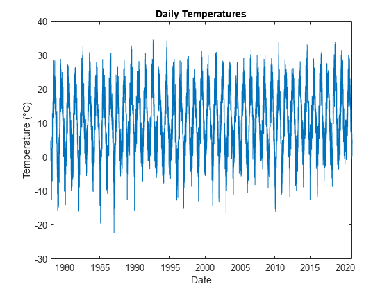
This example uses data containing temperatures from 1978 to the end of 2020 near Stockholm. You can obtain this data by using getGHCNData in Local Functions.
stationID = 'SW000008525';
Element = 'TMAX';
startDate = datetime(1978,1,1);
endDate = datetime(2020,12,31);
Temp = getGHCNData(stationID,Element,startDate,endDate,false)
Temp=15706×1 timetable
    01-Jan-1978     4.7000
    02-Jan-1978          5
    03-Jan-1978     3.1000
    04-Jan-1978    -0.5000
    05-Jan-1978    -1.2000
    06-Jan-1978     2.7000
    07-Jan-1978     4.5000
    08-Jan-1978     4.9000
    09-Jan-1978     1.8000
    10-Jan-1978     3.2000
    11-Jan-1978     1.5000
    12-Jan-1978    -0.5000
    13-Jan-1978     0.6000
    14-Jan-1978          2
      ⋮
Visualize Temperatures
Use plotTemperature in Local Functions to visualize the daily temperatures.
figure
plot( Temp.Date, Temp.TMAX)
xlabel("Date")
ylabel("Temperature (" + char(176) + "C)")
title("Daily Temperatures")
In the remaining sections of this example, you model the temperature and then evaluate sample option prices.
Determine Seasonality in Data
Assume that the deterministic component of the temperature model comprises a linear trend and seasonal terms. To estimate the main frequencies present in the time series, apply the Fourier transform.
Use determineSeasonality in Local Functions to remove the linear trend by subtracting the best-fit line. Then, use the periodogram (Signal Processing Toolbox) function to compute the spectrum (with a sample rate of one observation per day), and to visualize the spectrum. In addition, the determineSeasonality function identifies the top two component frequencies and periods in the data and adds these to the power spectrum.
determineSeasonality(Temp)
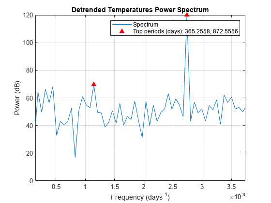
The plot illustrates that the dominant seasonal components in the data are the annual and 6-monthly cycles.
Fit Deterministic Trend
Based on the previous results, fit the following function for the temperature using the fitlm function.
elapsedTime = years(Temp.Date - Temp.Date(1));
designMatrix = @(t) [t, cos( 2 * pi * t ), sin( 2 * pi * t ), cos( 4 * pi * t )];
trendPreds = ["t", "cos(2*pi*t)", "sin(2*pi*t)", "cos(4*pi*t)"];
trendModel = fitlm(designMatrix(elapsedTime), Temp.TMAX, "VarNames", [trendPreds, "Temperature"])
trendModel =
Linear regression model:
    Temperature ~ 1 + t + cos(2*pi*t) + sin(2*pi*t) + cos(4*pi*t)

Estimated Coefficients:
                   Estimate       SE         tStat       pValue
                   ________    _________    _______    __________

    (Intercept)      9.7095     0.064138     151.39             0
    t              0.054648    0.0025836     21.152    6.1629e-98
    cos(2*pi*t)     -10.909     0.045348    -240.56             0
    sin(2*pi*t)      -2.772     0.045357    -61.115             0
    cos(4*pi*t)     0.39298     0.045348     8.6659    4.9102e-18


Number of observations: 15706, Error degrees of freedom: 15701
Root Mean Squared Error: 4.02
R-squared: 0.798,  Adjusted R-Squared: 0.798
F-statistic vs. constant model: 1.55e+04, p-value = 0
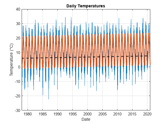
Use the plotDeterministicTrend in Local Functions to visualize the fitted trend.
trendModel = plotDeterministicTrend(Temp, trendModel, 1978, 2020)
trendModel =
Linear regression model:
    Temperature ~ 1 + t + cos(2*pi*t) + sin(2*pi*t) + cos(4*pi*t)

Estimated Coefficients:
                   Estimate       SE         tStat       pValue
                   ________    _________    _______    __________

    (Intercept)      9.7095     0.064138     151.39             0
    t              0.054648    0.0025836     21.152    6.1629e-98
    cos(2*pi*t)     -10.909     0.045348    -240.56             0
    sin(2*pi*t)      -2.772     0.045357    -61.115             0
    cos(4*pi*t)     0.39298     0.045348     8.6659    4.9102e-18


Number of observations: 15706, Error degrees of freedom: 15701
Root Mean Squared Error: 4.02
R-squared: 0.798,  Adjusted R-Squared: 0.798
F-statistic vs. constant model: 1.55e+04, p-value = 0
The coefficient of the term is significant with a value of 0.038. This value suggests that this geographic location has a warming trend of approximately 0.038°C per year.
Analyze and Fit Model Residuals
Create an ARIMA/GARCH model for the residuals using arima (Econometrics Toolbox).
Based on the preceding results, create a separate time-series model for the regression model residuals using the following workflow:
Create an
arima(Econometrics Toolbox) object and use theARMAterms help to model the autocorrelation in the residual series.Set the constant term to
0, since the regression model above already includes a constant.Use a -distribution for the innovation series.
Use a
garch(Econometrics Toolbox) model for the variance of the residuals to model the autocorrelation in the squared residuals.
trendRes = trendModel.Residuals.Raw;

resModel = arima( "ARLags", 1, ...
    "MALags", 1, ...
    "Constant", 0, ...
    "Distribution", "t", ...
    "Variance", garch( 1, 1 ) );
resModel = estimate(resModel,trendRes);
    ARIMA(1,0,1) Model (t Distribution):

                 Value      StandardError    TStatistic      PValue
                ________    _____________    __________    __________

    Constant           0              0           NaN             NaN
    AR{1}        0.76851      0.0063873        120.32               0
    MA{1}       0.075024       0.010201        7.3546      1.9155e-13
    DoF           10.369        0.75565        13.722        7.47e-43


    GARCH(1,1) Conditional Variance Model (t Distribution):

                 Value      StandardError    TStatistic      PValue
                ________    _____________    __________    __________

    Constant     0.67469       0.091762        7.3527      1.9427e-13
    GARCH{1}     0.82015       0.019319        42.452               0
    ARCH{1}     0.070965      0.0069394        10.226      1.5123e-24
    DoF           10.369        0.75565        13.722        7.47e-43
The residuals are not normally distributed or independent. Also, the residuals show evidence of GARCH effects.
Simulate Future Temperature Scenarios
Now that you have a calibrated temperature model, you can use it to simulate future temperature paths.
Prepare the simulation time.
nDays = 730;
simDates = Temp.Date(end) + caldays(1:nDays).';
simTime = years(simDates - Temp.Date(1));
Use predict to predict the deterministic trend.
trendPred = predict(trendModel, designMatrix(simTime));
Simulate from the ARIMA/GARCH model using simulate (Econometrics Toolbox).
simRes = simulate(resModel, nDays, "NumPaths", 1000, "Y0", trendRes);
Add the deterministic trend to the simulated residuals.
simTemp = simRes + trendPred;
Use visualizeScenarios in Local Functions to visualize the temperature scenarios.
visualizeScenarios(Temp, simTemp, simDates)

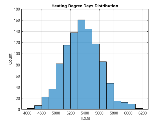
Evaluate Number of Heating Degree Days from Simulation
The number of heating degree days is given by , where are the simulated temperatures.
H = sum(max(18 - simTemp, 0));

figure
histogram(H)
xlabel("HDDs")
ylabel("Count")
title("Heating Degree Days Distribution")
grid on
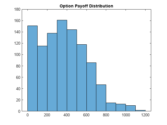
Using the original formula from Alaton [1], you can obtain a payoff distribution. When K = 7400, the max of H_n-K and 0 is always 0 for the set of simulation results in this example. Consequently, the histogram shows the distribution of 1000 zeros, that is, a single bar centered at 0 with a height of 1000. As K decreases to 5000, H_n-K has more opportunities to be positive, so the histogram changes shape.
K =5000; figure alpha = 1; chi = alpha*max(H-K, 0); % Payoff of option histogram(chi) title("Option Payoff Distribution")
Price Sample Call and Put Options
The weather derivative option pricing calculation is based on H (the number of heating degree days) which is defined in the Evaluate Number of Heating Degree Days From Simulation section.
First, compute the mean and standard deviation of H.
muH = mean(H);
sigmaH = std(H);
Define the sample option parameters.
r = 0.01; % Risk-free interest rate
K = 5000; % Strike value
TTM = 0.25; % Expiry time
Evaluate α.
a = (K - muH) / sigmaH;
Compute the price of the call and put options.
call_option = exp(-r*TTM) * ((muH - K) * normcdf(-a) + (sigmaH / sqrt(2*pi) * exp(-0.5*a^2)))
call_option =
370.4625
put_option = exp(-r*TTM) * ((K - muH) * (normcdf(a) - normcdf(-muH / sigmaH)) + sigmaH / sqrt(2*pi) * (exp(-0.5*a^2) - exp(-0.5*(muH/sigmaH)^2)))
put_option =
8.6969
References
[1] Alaton, P., Djehiche, B. and D. Stillberger, D. On Modelling and Pricing Weather Derivatives. Applied Mathematical Finance. 9(1): 1–20, 2002.
[2] Climate Data Online: Web Services Documentation at https://www.ncdc.noaa.gov/cdo-web/webservices.
Local Functions
function TT_out = getGHCNData(stationID,Element,startDate,endDate,useNOAAinterface)
% Function to retrieve GHCN Data

% Set flag to use NOAA interface
if ~exist("useNOAAinterface","var") || isempty(useNOAAinterface)
  useNOAAinterface = false;
end

% For more information on the NOAA interface, see
% https://www.mathworks.com/matlabcentral/fileexchange/119213-matlab-interface-for-noaa-data

% Get data using noaa interface or readtable from NOAA site
if useNOAAinterface
  n = noaa("WebServicesTokenString");

  % Must request data in 1 year increments
  yearRange = year([startDate;endDate]);
  TT_Full_From_NOAA = [];
  for y = yearRange(1):yearRange(2)
    TT_Full_Year = getdata(n,"GHCND",datetime(y,1,1),datetime(y,12,31),stationid = strcat("GHCND:",stationID),datatypeid = Element,limit = "1000");
    TT_Full_From_NOAA = vertcat(TT_Full_From_NOAA,TT_Full_Year);  %#ok
    Date = datetime(TT_Full_From_NOAA.date,"InputFormat",'uuuu-MM-dd''T''HH:mm:SS');
    TT_out = timetable(Date,TT_Full_From_NOAA.value/10,'VariableNames',{Element});
  end

else

  % Import options for GHCN Data files. For more information, see:
  % https://www1.ncdc.noaa.gov/pub/data/ghcn/daily/readme.txt
  DataStartLine = 1;
  NumVariables = 31*4 + 4;
  varNames_Array = (["Value","MFlag","QFlag","SFlag"] + (1:31)')';
  VariableNames  = ["ID","Year","Month","Element",varNames_Array(:)'];
  VariableWidths = [11 4 2 4 repmat([5 1 1 1],1,31)];
  DataType       = [{'char','double','double','char'} ...
      repmat({'double' 'char' 'char' 'char'},1,31)];
  opts = fixedWidthImportOptions('NumVariables',NumVariables, ...
      'DataLines',DataStartLine, ...
      'VariableNames',VariableNames, ...
      'VariableWidths',VariableWidths, ...
      'VariableTypes',DataType);

  % Read the full data set.
  TT_Full = readtable("https://www1.ncdc.noaa.gov/pub/data/ghcn/daily/all/" + ...
      stationID + ".dly",opts);

  % Extract the Element data.
  TT_Element_Full = TT_Full(TT_Full.Element == string(Element),["ID" "Year" ...
      "Month" "Element" "Value" + (1:31)]);

  reqYears = year(startDate):year(endDate);
  TT_Element = TT_Element_Full(ismember(TT_Element_Full.Year,reqYears),:);

  fullyearDays = datetime(year(startDate),1,1):datetime(year(endDate),12,31);

  tmpData = TT_Element{:,5:end}';
  tmpData = tmpData(:);
  tmpData(tmpData == -9999) = []; % Remove any empty data

  Date = (startDate:endDate)';
  reqIndex = ismember(fullyearDays,Date);
  TT_out = timetable(Date,tmpData(reqIndex)/10,'VariableNames',{Element});

end

end

function determineSeasonality(Temp)

% Assume that the deterministic component of the temperature model comprises a linear trend and seasonal terms.
% To estimate the main frequencies present in the time series, apply the Fourier transform.
% First, remove the linear trend by subtracting the best-fit line.

detrendedTemps = detrend(Temp.TMAX);

% Next, use the periodogram function to compute the spectrum. The sampling frequency is one observation per day.
numObs = length(detrendedTemps);
Fs = 1;
[pow, freq] = periodogram(detrendedTemps, [], numObs, Fs);

% Visualize the spectrum.
powdB = db(pow);
figure
plot(freq, powdB)
xlabel("Frequency (days^{-1})")
ylabel("Power (dB)")
title("Detrended Temperatures Power Spectrum")
grid on

% Identify the top two component frequencies and periods in the data.
[topPow, idx] = findpeaks(powdB, "NPeaks", 2, ...
    "SortStr", "descend", ...
    "MinPeakProminence", 20);
topFreq = freq(idx);
topPeriods = 1 ./ topFreq;

% Add the top two component frequencies and periods to the spectrum.
hold on
plot(topFreq, topPow, "r^", "MarkerFaceColor", "r")
xlim([min( topFreq ) - 1e-3, max( topFreq ) + 1e-3])
legend("Spectrum", "Top periods (days): " + join( string( topPeriods ), ", " ))
% Note that the dominant seasonal components in the data are the annual and 6-monthly cycles.

end

function trendModel = plotDeterministicTrend(Temp, trendModel, from, to)
% Visualize the fitted trend.
figure;
plot(Temp.Date, Temp.TMAX)
xlabel("Date")
ylabel("Temperature (" + char( 176 ) + "C)")
title("Daily Temperatures")
grid on
hold on
plot(Temp.Date, trendModel.Fitted, "LineWidth", 2)
plot(Temp.Date,6.06+0.038*years(Temp.Date - Temp.Date(1)),'k--','LineWidth',2)
xlim([datetime(from,1,1), datetime(to,12,31)])
end

function visualizeScenarios(Temp, simTemp, simDates)
figure
plot(Temp.Date, Temp.TMAX)
hold on
plot(simDates, simTemp)

% Plot the simulation percentiles.
simPrc = prctile(simTemp, [2.5, 50, 97.5], 2);
plot(simDates, simPrc, "y", "LineWidth", 1.5)
xlim([Temp.Date(end) - calyears(1), simDates(end)])
xlabel("Date")
ylabel("Temperature (" + char( 176 ) + "C)")
title("Temperature Simulation")
grid on

% Get the data for 2021.
stationID = 'SW000008525';
Element = 'TMAX';
startDate = datetime(2021,1,1);
endDate = datetime(2021,12,31);
T = getGHCNData(stationID,Element,startDate,endDate);
plot(T.Date,  T.TMAX, "g", "LineWidth", 1.5)

end