simulate

Monte Carlo simulation of univariate ARIMA or ARIMAX models

Syntax

Y = simulate(Mdl,numobs)

Y = simulate(Mdl,numobs,Name=Value)

[Y,E,V] = simulate(___)

Tbl = simulate(Mdl,numobs,Presample=Presample,PresampleResponseVariable=PresampleResponseVariable)

Tbl = simulate(Mdl,numobs,InSample=InSample,PredictorVariables=PredictorVariables)

Tbl = simulate(Mdl,numobs,Presample=Presample,PresampleResponseVariable=PresampleResponseVariable,InSample=InSample,PredictorVariables=PredictorVariables)

Tbl = simulate(___,Name=Value)

Description

Y = simulate(Mdl,numobs) returns the numeric vector Y containing a random numobs-period response path from simulating the fully specified ARIMA model Mdl.

Y = simulate(Mdl,numobs,Name=Value) uses additional options specified by one or more name-value arguments. simulate returns numeric arrays when all optional input data are numeric arrays. For example, simulate(Mdl,100,NumPaths=1000,Y0=PS) returns a numeric array of 1000, 100-period simulated response paths from Mdl and specifies the numeric array of presample response data PS.

[Y,E,V] = simulate(___) uses any input-argument combination in the previous syntaxes to return numeric arrays of one or more independent series of model innovations E and, when Mdl represents a composite conditional mean and variance model, conditional variances V, resulting from simulating the ARIMA model.

Tbl = simulate(Mdl,numobs,Presample=Presample,PresampleResponseVariable=PresampleResponseVariable) returns the table or timetable Tbl containing a variable for each of the random paths of response, innovation, and conditional variance series resulting from simulating the ARIMA model Mdl. simulate uses the response variable PresampleResponseVariable in the table or timetable of presample data Presample to initialize the response series. (since R2023b)

To initialize the model using presample innovation or conditional variance data, replace the PresampleResponseVariable name-value argument with PresampleInnovationVariable or PresampleVarianceVariable name-value argument.

Tbl = simulate(Mdl,numobs,InSample=InSample,PredictorVariables=PredictorVariables) specifies the variables PredictorVariables in the in-sample table or timetable of data InSample containing the predictor data for the exogenous regression component in the ARIMA model Mdl. (since R2023b)

Tbl = simulate(Mdl,numobs,Presample=Presample,PresampleResponseVariable=PresampleResponseVariable,InSample=InSample,PredictorVariables=PredictorVariables) specifies presample response data to initialize the model and in-sample predictor data for the exogenous regression component. (since R2023b)

Tbl = simulate(___,Name=Value) uses additional options specified by one or more name-value arguments, using any input argument combination in the previous three syntaxes. (since R2023b)

For example, simulate(Mdl,100,NumPaths=1000,Presample=PSTbl,PresampleResponseVariables="GDP") returns a timetable containing a variable for each of the response, innovations, and conditional variance series. Each variable is a 100-by-1000 matrix representing 1000, 100-period paths simulated from the ARIMA model. simulate initializes the model by using the presample data in the GDP variable of the timetable PSTbl.

Examples

Return Vector of Simulated Response Path from ARIMA Model

Simulate a response path from an ARIMA model. Return the path in a vector.

Consider the ARIMA(4,1,1) model

$$(1-0.75L^4)(1-L)y_t=2+(1+0.1L){\epsilon }_t,$$

where ${\epsilon }_{\mathit{t}}$ is a Gaussian innovations series with a mean of 0 and a variance of 1.

Create the ARIMA(4,1,1) model.

Mdl = arima(AR=-0.75,ARLags=4,MA=0.1,Constant=2,Variance=1)

Mdl = 
  arima with properties:

     Description: "ARIMA(4,0,1) Model (Gaussian Distribution)"
      SeriesName: "Y"
    Distribution: Name = "Gaussian"
               P: 4
               D: 0
               Q: 1
        Constant: 2
              AR: {-0.75} at lag [4]
             SAR: {}
              MA: {0.1} at lag [1]
             SMA: {}
     Seasonality: 0
            Beta: [1×0]
        Variance: 1

Mdl is a fully specified arima object representing the ARIMA(4,1,1) model.

Simulate a 100-period random response path from the ARIMA(4,1,1) model.

rng(1,"twister")  % For reproducibility
y = simulate(Mdl,100);

y is a 100-by-1 vector containing the random response path.

Plot the simulated path.

plot(y)
ylabel("y")
xlabel("Time")

Simulate Predictors and Responses

Simulate three predictor series and a response series.

Specify and simulate a path of length 20 for each of the three predictor series modeled by

$$(1-0.2L)x_{it}=2+(1+0.5L-0.3L^2){\eta }_{it},$$

where $${\eta }_{it}$$ follows a Gaussian distribution with mean 0 and variance 0.01, and $$i$$ = {1,2,3}.

[MdlX1,MdlX2,MdlX3] = deal(arima(AR=0.2,MA={0.5 -0.3}, ...
    Constant=2,Variance=0.01));

rng(4,"twister"); % For reproducibility 
simX1 = simulate(MdlX1,20);
simX2 = simulate(MdlX2,20);
simX3 = simulate(MdlX3,20);
SimX = [simX1 simX2 simX3];

Specify and simulate a path of length 20 for the response series modeled by

$$(1-0.05L+0.02L^2-0.01L^3)(1-L{)}^1{y}_t=0.05+x_t^{\prime }\left[\begin{array}{c}0.5\\ -0.03\\ -0.7\end{array}\right]+(1+0.04L+0.01L^2){\epsilon }_t,$$

where $${\epsilon }_t$$ follows a Gaussian distribution with mean 0 and variance 1.

MdlY = arima(AR={0.05 -0.02 0.01},MA={0.04 0.01}, ...
    D=1,Constant=0.5,Variance=1,Beta=[0.5 -0.03 -0.7]);
simY = simulate(MdlY,20,X=SimX);

Plot the series together.

figure
plot([SimX simY])
title("Simulated Series")
legend("x_1","x_2","x_3","y")

Forecast Process Using Simulations

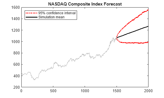
Forecast the daily NASDAQ Composite Index using Monte Carlo simulations. Supply presample observations to initialize the model.

Load the NASDAQ data included with the toolbox. Extract the first 1500 observations for fitting.

load Data_EquityIdx
nasdaq = DataTable.NASDAQ(1:1500);
T = length(nasdaq);

Fit an ARIMA(1,1,1) model.

NasdaqModel = arima(1,1,1);
NasdaqFit = estimate(NasdaqModel,nasdaq);

 
    ARIMA(1,1,1) Model (Gaussian Distribution):
 
                  Value      StandardError    TStatistic      PValue  
                _________    _____________    __________    __________

    Constant      0.43031       0.18555           2.319       0.020393
    AR{1}       -0.074391      0.081985        -0.90737        0.36421
    MA{1}         0.31126      0.077266          4.0284     5.6158e-05
    Variance       27.826       0.63625          43.735              0

Simulate 1000 paths with 500 observations each. Use the observed data as presample data.

rng(1,"twister");
Y = simulate(NasdaqFit,500,NumPaths=1000,Y0=nasdaq);

Plot the simulation mean forecast and approximate 95% forecast intervals.

lower = prctile(Y,2.5,2);
upper = prctile(Y,97.5,2);
mn = mean(Y,2);
x = T + (1:500);
figure
plot(nasdaq,Color=[.7,.7,.7])
hold on
h1 = plot(x,lower,"r:",LineWidth=2);
plot(x,upper,"r:",LineWidth=2)
h2 = plot(x,mn,"k",LineWidth=2);
legend([h1 h2],"95% confidence interval","Simulation mean", ...
    Location="NorthWest")
title("NASDAQ Composite Index Forecast")
hold off

Simulate Responses and Innovations

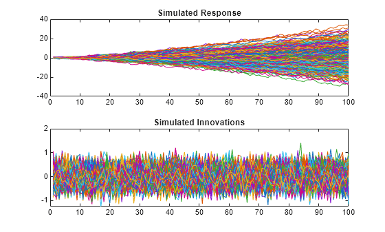
Simulate response and innovation paths from a multiplicative seasonal model.

Specify the model

$$(1-L)(1-L^{12})y_t=(1-0.5L)(1+0.3L^{12}){\epsilon }_t,$$

where $${\epsilon }_t$$ follows a Gaussian distribution with mean 0 and variance 0.1.

Mdl = arima(MA=-0.5,SMA=0.3,SMALags=12,D=1, ...
    Seasonality=12,Variance=0.1,Constant=0);

Simulate 500 paths with 100 observations each.

rng(1,"twister") % For reproducibility
[Y,E] = simulate(Mdl,100,NumPaths=500);

figure
tiledlayout(2,1)
nexttile
plot(Y)
title("Simulated Response")
nexttile
plot(E)
title("Simulated Innovations")

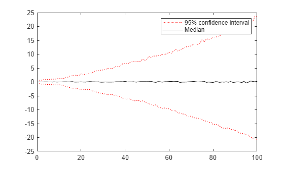
Plot the 2.5th, 50th (median), and 97.5th percentiles of the simulated response paths.

lower = prctile(Y,2.5,2);
middle = median(Y,2);
upper = prctile(Y,97.5,2);

figure
plot(1:100,lower,"r:",1:100,middle,"k", ...
    1:100,upper,"r:")
legend("95% confidence interval","Median")

Compute statistics across the second dimension (across paths) to summarize the sample paths.

Plot a histogram of the simulated paths at time 100.

figure
histogram(Y(100,:),10)
title("Response Distribution at Time 100")

Supply Presample Data in Timetable

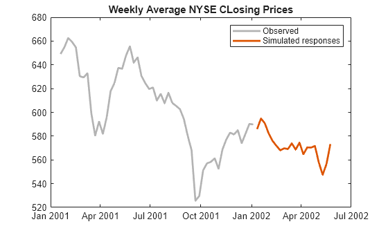
Fit an ARIMA(1,1,1) model to the weekly average NYSE closing prices. Supply a timetable of presample responses to initialize the model and return a timetable of simulated values from the model.

Load Data

Load the US equity index data set Data_EquityIdx.

load Data_EquityIdx
T = height(DataTimeTable)

T = 
3028

The timetable DataTimeTable includes the time series variable NYSE, which contains daily NYSE composite closing prices from January 1990 through December 2001.

Plot the daily NYSE price series.

figure
plot(DataTimeTable.Time,DataTimeTable.NYSE)
title("NYSE Daily Closing Prices: 1990 - 2001")

Prepare Timetable for Estimation

When you plan to supply a timetable, you must ensure it has all the following characteristics:

• The selected response variable is numeric and does not contain any missing values.

• The timestamps in the Time variable are regular, and they are ascending or descending.

Remove all missing values from the timetable, relative to the NYSE price series.

DTT = rmmissing(DataTimeTable,DataVariables="NYSE");
T_DTT = height(DTT)

T_DTT = 
3028

Because all sample times have observed NYSE prices, rmmissing does not remove any observations.

Determine whether the sampling timestamps have a regular frequency and are sorted.

areTimestampsRegular = isregular(DTT,"days")

areTimestampsRegular = logical
   0

areTimestampsSorted = issorted(DTT.Time)

areTimestampsSorted = logical
   1

areTimestampsRegular = 0 indicates that the timestamps of DTT are irregular. areTimestampsSorted = 1 indicates that the timestamps are sorted. Business day rules make daily macroeconomic measurements irregular.

Remedy the time irregularity by computing the weekly average closing price series of all timetable variables.

DTTW = convert2weekly(DTT,Aggregation="mean");
areTimestampsRegular = isregular(DTTW,"weeks")

areTimestampsRegular = logical
   1

T_DTTW = height(DTTW)

T_DTTW = 
627

DTTW is regular.

figure
plot(DTTW.Time,DTTW.NYSE)
title("NYSE Daily Closing Prices: 1990 - 2001")

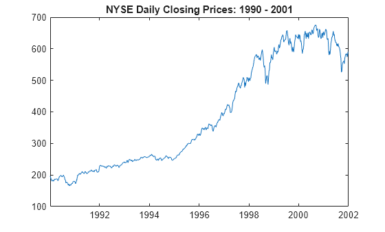
Create Model Template for Estimation

Suppose that an ARIMA(1,1,1) model is appropriate to model NYSE composite series during the sample period.

Create an ARIMA(1,1,1) model template for estimation.

Mdl = arima(1,1,1);

Mdl is a partially specified arima model object.

Fit Model to Data

infer requires Mdl.P presample observations to initialize the model. infer backcasts for necessary presample responses, but you can provide a presample.

Partition the data into presample and in-sample, or estimation sample, observations.

T0 = Mdl.P;
DTTW0 = DTTW(1:T0,:);
DTTW1 = DTTW((T0+1):end,:);

Fit an ARIMA(1,1,1) model to the in-sample weekly average NYSE closing prices. Specify the response variable name, presample timetable, and the presample response variable name.

EstMdl = estimate(Mdl,DTTW1,ResponseVariable="NYSE", ...
    Presample=DTTW0,PresampleResponseVariable="NYSE");

 
    ARIMA(1,1,1) Model (Gaussian Distribution):
 
                 Value      StandardError    TStatistic      PValue   
                ________    _____________    __________    ___________

    Constant     0.83623         0.453          1.846         0.064892
    AR{1}       -0.32862       0.23526        -1.3968          0.16246
    MA{1}        0.42703       0.22613         1.8885         0.058964
    Variance      56.065        1.8433         30.416      3.3806e-203

EstMdl is a fully specified, estimated arima model object.

Simulate Model

Simulate the fitted model 20 weeks beyond the final period. Specify the entire in-sample data as a presample and the presample response variable name in the in-sample timetable.

rng(1,"twister")    % For reproducibility
numobs = 20;
Tbl = simulate(EstMdl,numobs,Presample=DTTW1, ...
    PresampleResponseVariable="NYSE");
tail(Tbl)

       Time        Y_Response    Y_Innovation    Y_Variance
    ___________    __________    ____________    __________

    05-Apr-2002      564.68        -11.302         56.065  
    12-Apr-2002      570.47         6.5582         56.065  
    19-Apr-2002      570.39        -1.8179         56.065  
    26-Apr-2002      571.72          1.249         56.065  
    03-May-2002      557.94        -14.716         56.065  
    10-May-2002      547.51        -9.5098         56.065  
    17-May-2002      556.51         8.7992         56.065  
    24-May-2002      573.34         15.194         56.065  

size(Tbl)

ans = 1×2

    20     3

Tbl is a 20-by-3 timetable containing the simulated response path NYSE_Response, the corresponding simulated innovation path NYSE_Innovation, and the constant variance path NYSE_Variance (Mdl.Variance = 56.065).

Plot the simulated responses.

figure
plot(DTTW1.Time((end-50):end),DTTW1.NYSE((end-50):end), ...
    Color=[0.7 0.7 0.7],LineWidth=2);
hold on
plot(Tbl.Time,Tbl.Y_Response,LineWidth=2);
legend("Observed","Simulated responses")
title("Weekly Average NYSE CLosing Prices")
hold off

Supply Timetable of Presample and Predictor Data

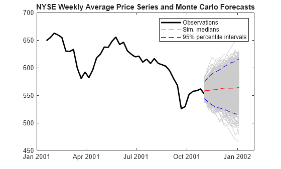
Fit an ARIMAX(1,1,1) model to the weekly average NYSE closing prices. Include an exogenous regression term identifying whether a measurement observation occurs during a recession. Supply timetables of presample and in-sample exogenous data. Simulate the weekly average closing prices over a 10-week horizon, and compare the forecasts to held out data.

Load the US equity index data set Data_EquityIdx.

load Data_EquityIdx
T = height(DataTimeTable)

T = 
3028

Remedy the time irregularity by computing the weekly average closing price series of all timetable variables.

DTTW = convert2weekly(DataTimeTable,Aggregation="mean");
T_DTTW = height(DTTW)

T_DTTW = 
627

Load the US recessions data set.

load Data_Recessions
RDT = datetime(Recessions,ConvertFrom="datenum", ...
    Format="yyyy-MM-dd");

Determine whether each sampling time in the data occurs during a US recession.

isrecession = @(x)any(isbetween(x,RDT(:,1),RDT(:,2)));
DTTW.IsRecession = arrayfun(isrecession,DTTW.Time)*1;

DTTW contains a variable IsRecession, which represents the exogenous variable in the ARIMAX model.

Create an ARIMA(1,1,1) model template for estimation. Set the response series name to NYSE.

Mdl = arima(1,1,1);
Mdl.SeriesName = "NYSE";

Partition the data into required presample, in-sample (estimation sample), and 10 holdout sample observations.

T0 = Mdl.P;
T2 = 10;
DTTW0 = DTTW(1:T0,:);
DTTW1 = DTTW((T0+1):(end-T2),:);
DTTW2 = DTTW((end-T2+1):end,:);

Fit an ARIMA(1,1,1) model to the in-sample weekly average NYSE closing prices. Specify the presample timetable, the presample response variable name, and the in-sample predictor variable name.

EstMdl = estimate(Mdl,DTTW1,Presample=DTTW0,PresampleResponseVariable="NYSE", ...
    PredictorVariables="IsRecession");

 
    ARIMAX(1,1,1) Model (Gaussian Distribution):
 
                 Value      StandardError    TStatistic      PValue   
                ________    _____________    __________    ___________

    Constant      1.0635       0.50013         2.1264         0.033468
    AR{1}       -0.33828        0.2088        -1.6201           0.1052
    MA{1}        0.43879       0.20045          2.189         0.028593
    Beta(1)       -2.425        1.0861        -2.2327          0.02557
    Variance      55.527        1.9255         28.838      7.0988e-183

Simulate 1000 paths of responses from the fitted model into a 10-week horizon. Specify the in-sample data as a presample, the presample response variable name, the predictor data in the forecast horizon, and the predictor variable name.

rng(1,"twister")
Tbl = simulate(EstMdl,T2,Presample=DTTW1,PresampleResponseVariable="NYSE", ...
    InSample=DTTW2,PredictorVariables="IsRecession",NumPaths=1000);

Tbl is a 10-by-6 timetable containing all variables in InSample, and the following variables:

• NYSE_Response: a 10-by-1000 matrix of 1000 random response paths simulated from the model.

• NYSE_Innovation: a 10-by-1000 matrix of 1000 random innovation paths filtered through the model to product the response paths

• NYSE_Variance: a 10-by-1000 matrix containing only the constant Mdl.Variance = 55.527.

Plot the observed responses, median of the simulated responses, a 95% percentile intervals of the simulated values.

SimStats = quantile(Tbl.NYSE_Response,[0.025 0.5 0.975],2);

figure
h1 = plot(DTTW.Time((end-50):end),DTTW.NYSE((end-50):end),"k",LineWidth=2);
hold on
plot(Tbl.Time,Tbl.NYSE_Response,Color=[0.8 0.8 0.8])
h2 = plot(Tbl.Time,SimStats(:,2),'r--');
h3 = plot(Tbl.Time,SimStats(:,[1 3]),'b--');
legend([h1 h2 h3(1)],["Observations" "Sim. medians" "95% percentile intervals"])
title("NYSE Weekly Average Price Series and Monte Carlo Forecasts")

Input Arguments

Mdl — Fully specified ARIMA model

arima model object

Fully specified ARIMA model, specified as an arima model object created by arima or estimate.

The properties of Mdl cannot contain NaN values.

numobs — Sample path length

positive integer

Sample path length, specified as a positive integer. numobs is the number of random observations to generate per output path.

Data Types: double

Presample — Presample data

table | timetable

Since R2023b

Presample data containing paths of responses y_t, innovations ε_t, or conditional variances σ_t² to initialize the model, specified as a table or timetable with numprevars variables and numpreobs rows.

simulate returns the simulated variables in the output table or timetable Tbl, which is the same type as Presample. If Presample is a timetable, Tbl is a timetable that immediately follows Presample in time with respect to the sampling frequency.

Each selected variable is a single path (numpreobs-by-1 vector) or multiple paths (numpreobs-by-numprepaths matrix) of numpreobs observations representing the presample of numpreobs observations of responses, innovations, or conditional variances.

Each row is a presample observation, and measurements in each row occur simultaneously. The last row contains the latest presample observation. numpreobs must be one of the following values:

• At least Mdl.P when Presample provides only presample responses

• At least Mdl.Q when Presample provides only presample disturbances or conditional variances

• At least max([Mdl.P Mdl.Q]) otherwise

When Mdl.Variance is a conditional variance model, simulate can require more than the minimum required number of presample values.

If numpreobs exceeds the minimum number, simulate uses the latest required number of observations only.

If numprepaths > NumPaths, simulate uses only the first NumPaths columns.

If Presample is a timetable, all the following conditions must be true:

• Presample must represent a sample with a regular datetime time step (see isregular).

• The datetime vector of sample timestamps Presample.Time must be ascending or descending.

• If you specify InSample, Presample must immediately precede InSample, with respect to the sampling frequency.

If Presample is a table, the last row contains the latest presample observation.

By default, simulate sets the following values:

• For necessary presample responses:

  • The unconditional mean of the model when Mdl represents a stationary AR process without a regression component

  • Zero when Mdl represents a nonstationary process or when it contains a regression component.

• For necessary presample disturbances, zero.

• For necessary presample conditional variances, the unconditional variance of the conditional variance model n Mdl.Variance.

If you specify the Presample, you must specify the presample response, innovation, or conditional variance variable name by using the PresampleResponseVariable, PresampleInnovationVariable, or PresampleVarianceVariable name-value argument.

PresampleResponseVariable — Response variable y_t to select from Presample

string scalar | character vector | integer | logical vector

Since R2023b

Response variable y_t to select from Presample containing presample response data, specified as one of the following data types:

• String scalar or character vector containing a variable name in Presample.Properties.VariableNames

• Variable index (positive integer) to select from Presample.Properties.VariableNames

• A logical vector, where PresampleResponseVariable(j) = true selects variable j from Presample.Properties.VariableNames

The selected variable must be a numeric matrix and cannot contain missing values (NaNs).

If you specify presample response data by using the Presample name-value argument, you must specify PresampleResponseVariable.

Example: PresampleResponseVariable="Stock0"

Example: PresampleResponseVariable=[false false true false] or PresampleResponseVariable=3 selects the third table variable as the presample response variable.

Data Types: double | logical | char | cell | string

InSample — In-sample predictor data

table | timetable

Since R2023b

In-sample predictor data for the exogenous regression component of the model, specified as a table or timetable. InSample contains numvars variables, including numpreds predictor variables x_t.

simulate returns the simulated variables in the output table or timetable Tbl, which is commensurate with InSample.

Each row corresponds to an observation in the simulation horizon, the first row is the earliest observation, and measurements in each row, among all paths, occur simultaneously. InSample must have at least numobs rows to cover the simulation horizon. If you supply more rows than necessary, simulate uses only the first numobs rows.

Each selected predictor variable is a numeric vector without missing values (NaNs). All predictor variables are present in the regression component of each response equation and apply to all response paths.

If InSample is a timetable, the following conditions apply:

• InSample must represent a sample with a regular datetime time step (see isregular).

• The datetime vector InSample.Time must be ascending or descending.

• If you specify Presample, Presample must immediately precede InSample, with respect to the sampling frequency.

If InSample is a table, the last row contains the latest observation.

By default, simulate does not include the regression component in the model, regardless of the value of Mdl.Beta.

PredictorVariables — Exogenous predictor variables x_t to select from InSample

string vector | cell vector of character vectors | vector of integers | logical vector

Exogenous predictor variables x_t to select from InSample containing predictor data for the regression component, specified as one of the following data types:

• String vector or cell vector of character vectors containing numpreds variable names in InSample.Properties.VariableNames

• A vector of unique indices (positive integers) of variables to select from InSample.Properties.VariableNames

• A logical vector, where PredictorVariables(j) = true selects variable j from InSample.Properties.VariableNames

The selected variables must be numeric vectors and cannot contain missing values (NaNs).

By default, simulate excludes the regression component, regardless of its presence in Mdl.

Example: PredictorVariables=["M1SL" "TB3MS" "UNRATE"]

Example: PredictorVariables=[true false true false] or PredictorVariable=[1 3] selects the first and third table variables to supply the predictor data.

Data Types: double | logical | char | cell | string

Name-Value Arguments

Specify optional pairs of arguments as Name1=Value1,...,NameN=ValueN, where Name is the argument name and Value is the corresponding value. Name-value arguments must appear after other arguments, but the order of the pairs does not matter.

Before R2021a, use commas to separate each name and value, and enclose Name in quotes.

Example: simulate(Mdl,10,NumPaths=1000,Y0=y0) simulates 1000 sample paths of length 10 from the ARIMA model Mdl, and uses the observations in y0 as a presample to initialize each generated path.

NumPaths — Number of independent sample paths to generate

1 (default) | positive integer

Number of independent sample paths to generate, specified as a positive integer.

Example: NumPaths=1000

Data Types: double

Y0 — Presample response data y_t

numeric column vector | numeric matrix

Presample response data y_t used as initial values for the model, specified as a numpreobs-by-1 numeric column vector or a numpreobs-by-numprepaths numeric matrix. Use Y0 only when you supply optional data inputs as numeric arrays.

numpreobs is the number of presample observations. numprepaths is the number of presample response paths.

Each row is a presample observation (sampling time), and measurements in each row occur simultaneously. The last row contains the latest presample observation. numpreobs must be at least Mdl.P to initialize the AR model component. If numpreobs > Mdl.P, simulate uses the latest required number of observations only.

Columns of Y0 are separate, independent presample paths. The following conditions apply:

• If Y0 is a column vector, it represents a single response path. simulate applies it to each output path.

• If Y0 is a matrix, simulate applies Y0(:,j) to initialize path j. Y0 must have at least NumPaths columns; simulate uses only the first NumPaths columns of Y0.

By default, simulate sets any necessary presample responses to one of the following values:

• The unconditional mean of the model when Mdl represents a stationary AR process without a regression component

• Zero when Mdl represents a nonstationary process or when it contains a regression component

Data Types: double

E0 — Presample innovation data ε_t

numeric column vector | numeric matrix

Presample innovation data ε_t used to initialize either the moving average (MA) component of the ARIMA model or the conditional variance model, specified as a numpreobs-by-1 numeric column vector or a numpreobs-by-numprepaths matrix. Use E0 only when you supply optional data inputs as numeric arrays.

Each row is a presample observation (sampling time), and measurements in each row occur simultaneously. The last row contains the latest presample observation. numpreobs must be at least Mdl.Q to initialize the MA model component. If Mdl.Variance is a conditional variance model (for example, a garch model object), simulate can require more rows than Mdl.Q. If numpreobs is larger than required, simulate uses the latest required number of observations only.

Columns of E0 are separate, independent presample paths. The following conditions apply:

• If E0 is a column vector, it represents a single residual path. simulate applies it to each output path.

• If E0 is a matrix, simulate applies E0(:,j) to initialize simulating path j. E0 must have at least NumPaths columns; simulate uses only the first NumPaths columns of E0.

By default, simulate sets the necessary presample disturbances to zero.

Data Types: double

V0 — Presample conditional variance data σ_t²

positive numeric column vector | positive numeric matrix

Presample conditional variance data σ_t² used to initialize the conditional variance model, specified as a numpreobs-by-1 positive numeric column vector or a numpreobs-by-numprepaths positive numeric matrix. If the conditional variance Mdl.Variance is constant, simulate ignores V0. Use V0 only when you supply optional data inputs as numeric arrays.

Each row is a presample observation (sampling time), and measurements in each row occur simultaneously. The last row contains the latest presample observation. numpreobs must be at least Mdl.Q to initialize the conditional variance model in Mdl.Variance. For details, see the simulate function of conditional variance models. If numpreobs is larger than required, simulate uses the latest required number of observations only.

Columns of V0 are separate, independent presample paths. The following conditions apply:

• If V0 is a column vector, it represents a single path of conditional variances. simulate applies it to each output path.

• If V0 is a matrix, simulate applies V0(:,j) to initialize simulating path j. V0 must have at least NumPaths columns; simulate uses only the first NumPaths columns of V0.

By default, simulate sets all necessary presample observations to the unconditional variance of the conditional variance process.

Data Types: double

PresampleInnovationVariable — Residual variable e_t to select from Presample

string scalar | character vector | integer | logical vector

Since R2023b

Residual variable e_t to select from Presample containing the presample residual data, specified as one of the following data types:

• String scalar or character vector containing a variable name in Presample.Properties.VariableNames

• Variable index (positive integer) to select from Presample.Properties.VariableNames

• A logical vector, where PresampleInnovationVariable(j) = true selects variable j from Presample.Properties.VariableNames

The selected variable must be a numeric matrix and cannot contain missing values (NaNs).

If you specify presample residual data by using the Presample name-value argument, you must specify PresampleInnovationVariable.

Example: PresampleInnovationVariable="StockRateDist0"

Example: PresampleInnovationVariable=[false false true false] or PresampleInnovationVariable=3 selects the third table variable as the presample innovation variable.

Data Types: double | logical | char | cell | string

PresampleVarianceVariable — Conditional variance variable σ_t² to select from Presample

string scalar | character vector | integer | logical vector

Since R2023b

Conditional variance variable σ_t² to select from Presample containing presample conditional variance data, specified as one of the following data types:

• String scalar or character vector containing a variable name in Presample.Properties.VariableNames

• Variable index (positive integer) to select from Presample.Properties.VariableNames

• A logical vector, where PresampleVarianceVariable(j) = true selects variable j from Presample.Properties.VariableNames

The selected variable must be a numeric vector and cannot contain missing values (NaNs).

If you specify presample conditional variance data by using the Presample name-value argument, you must specify PresampleVarianceVariable.

Example: PresampleVarianceVariable="StockRateVar0"

Example: PresampleVarianceVariable=[false false true false] or PresampleVarianceVariable=3 selects the third table variable as the presample conditional variance variable.

Data Types: double | logical | char | cell | string

X — Exogenous predictor data

numeric matrix

Exogenous predictor data for the regression component in the model, specified as a numeric matrix with numpreds columns. numpreds is the number of predictor variables (numel(Mdl.Beta)). Use X only when you supply optional data inputs as numeric arrays.

Each row of X corresponds to a period in the length numobs simulation sample (period for which simulate simulates observations; the period after the presample). X must have at least numobs rows. The last row contains the latest predictor data. If X has more than numobs rows, simulate uses only the latest numobs rows.

simulate does not use the regression component in the presample period.

Columns of X are separate predictor variables.

simulate applies X to each simulated path; that is, X represents one path of observed predictors.

By default, simulate excludes the regression component, regardless of its presence in Mdl.

Data Types: double

Note

• NaN values in X, Y0, E0, and V0 indicate missing values. simulate removes missing values from specified data by list-wise deletion.

  • For the presample, simulate horizontally concatenates the possibly jagged arrays Y0, E0, and V0 with respect to the last rows, and then it removes any row of the concatenated matrix containing at least one NaN.

  • For in-sample data, simulate removes any row of X containing at least one NaN.

  This type of data reduction reduces the effective sample size and can create an irregular time series.

• For numeric data inputs, simulate assumes that you synchronize the presample data such that the latest observations occur simultaneously.

• simulate issues an error when any table or timetable input contains missing values.

Output Arguments

Y — Simulated response paths y_t

numeric column vector | numeric matrix

Simulated response paths y_t, returned as a numobs-by-1 numeric column vector or a numobs-by-NumPaths numeric matrix. simulate returns Y by default and when you supply optional data in numeric arrays.

Y represents the continuation of the presample responses in Y0.

Each row corresponds to a period in the simulated series; the simulated series has the periodicity of Mdl. Each column is a separate simulated path.

E — Simulated model innovations paths ε_t

numeric column vector | numeric matrix

Simulated model innovations paths ε_t, returned as a numobs-by-1 numeric column vector or a numobs-by-NumPaths numeric matrix. simulate returns E by default and when you supply optional data in numeric arrays

The dimensions of E correspond to the dimensions of Y.

V — Simulated conditional variance paths σ_t²

numeric column vector | numeric matrix

Simulated conditional variance paths σ_t² of the mean-zero innovations associated with Y, returned as a numobs-by-1 numeric column vector or a numobs-by-NumPaths numeric matrix. simulate returns V by default and when you supply optional data in numeric arrays

The dimensions of V correspond to the dimensions of Y.

Tbl — Simulated response y_t, innovation ε_t, and conditional variance σ_t² paths

table | timetable

Since R2023b

Simulated response y_t, innovation ε_t, and conditional variance σ_t² paths, returned as a table or timetable, the same data type as Presample or InSample. simulate returns Tbl only when you supply at least one of the inputs Presample and InSample.

Tbl contains the following variables:

• The simulated response paths, which are in a numobs-by-NumPaths numeric matrix, with rows representing observations and columns representing independent paths. Each path represents the continuation of the corresponding presample path in Presample, or each path corresponds, in time, with the rows of InSample. simulate names the simulated response variable in Tbl responseName_Response, where responseName is Mdl.SeriesName. For example, if Mdl.SeriesName is StockReturns, Tbl contains a variable for the corresponding simulated response paths with the name StockReturns_Response.

• The simulated innovation paths, which are in a numobs-by-NumPaths numeric matrix, with rows representing observations and columns representing independent paths. Each path represents the continuation of the corresponding presample path in Presample, or each path corresponds, in time, with the rows of InSample. simulate names the simulated innovation variable in Tbl responseName_Innovation, where responseName is Mdl.SeriesName. For example, if Mdl.SeriesName is StockReturns, Tbl contains a variable for the corresponding simulated innovation paths with the name StockReturns_Innovation.

• The simulated conditional variance paths, which are in a numobs-by-NumPaths numeric matrix, with rows representing observations and columns representing independent paths. Each path represents the continuation of the corresponding presample path in Presample, or each path corresponds, in time, with the rows of InSample. simulate names the simulated conditional variance variable in Tbl responseName_Variance, where responseName is Mdl.SeriesName. For example, if Mdl.SeriesName is StockReturns, Tbl contains a variable for the corresponding simulated conditional variance paths with the name StockReturns_Variance.

• When you supply InSample, Tbl contains all variables in InSample.

If Tbl is a timetable, the following conditions hold:

• The row order of Tbl, either ascending or descending, matches the row order of Preample.

• If you specify InSample, row times Tbl.Time are InSample.Time(1:numobs). Otherwise, Tbl.Time(1) is the next time after Presample(end) relative to the sampling frequency, and Tbl.Time(2:numobs) are the following times relative to the sampling frequency.

References

[1] Box, George E. P., Gwilym M. Jenkins, and Gregory C. Reinsel. Time Series Analysis: Forecasting and Control. 3rd ed. Englewood Cliffs, NJ: Prentice Hall, 1994.

[2] Enders, Walter. Applied Econometric Time Series. Hoboken, NJ: John Wiley & Sons, Inc., 1995.

[3] Hamilton, James D. Time Series Analysis. Princeton, NJ: Princeton University Press, 1994.

Version History

Introduced in R2012a

R2023a: simulate accepts input data in tables and timetables, and returns results in tables and timetables

In addition to accepting presample and in-sample predictor data in numeric arrays, simulate accepts input data in tables or regular timetables. When you supply input data in a table or timetable, the following conditions apply:

• If you specify optional presample response, innovation, or conditional variance data to initialize the model, you must also specify corresponding variable names containing the data to use.

• If you specify optional in-sample predictor data for the exogenous regression component of the model, you must also specify corresponding predictor variable names containing the data to use.

• simulate returns results in a table or timetable.

Name-value arguments to support tabular workflows include:

• Presample specifies the input table or regular timetable of presample innovations and conditional variance data.

• PresampleResponseVariable specifies the variable name of the response paths to select from Presample.

• PresampleInnovationVariable specifies the variable name of the innovation paths to select from Presample.

• PresampleVarianceVariable specifies the variable name of the conditional variance paths to select from Presample.

• InSample specifies the input table or regular timetable of in-sample predictor data.

• PredictorVariables specifies the names of the predictor series to select from InSample for a model regression component.