Hedging Using CVaR Portfolio Optimization
This example shows how to model two hedging strategies using CVaR portfolio optimization with a PortfolioCVaR object. First, you simulate the price movements of a stock by using a gbm object with simByEuler. Then you use CVaR portfolio optimization to estimate the efficient frontier of the portfolios for the returns at the horizon date. Finally, you compare the CVaR portfolio to a mean-variance portfolio to demonstrate the differences between these two types of risk measures.
Monte Carlo Simulation of Asset Scenarios
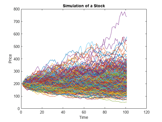
Scenarios are required to define and evaluate the CVaR portfolio. These scenarios can be generated in multiple ways, as well as obtained from historical observations. This example uses a Monte Carlo simulation of a geometric Brownian motion to generate the scenarios. The Monte Carlo simulation produces trials of a stock price after one year. These stock prices provide the returns of five different investment strategies that define the assets in the CVaR portfolio. This scenario generation strategy can be further generalized to simulations with more stocks, instruments, and strategies.
Define a stock profile.
% Price at time 0
Price_0 = 200;

% Drift (annualized)
Drift = 0.08;

% Volatility (annualized)
Vol = 0.4;

% Valuation date
Valuation = datetime(2012,1,1);

% Investment horizon date
Horizon = datetime(2013,1,1);

% Risk-free rate
RiskFreeRate = 0.03;
Simulate the price movements of the stock from the valuation date to the horizon date using a gbm object with simByEuler.
% Number of trials for the Monte Carlo simulation
NTRIALS = 100000;

% Length (in years) of the simulation
T = date2time(Valuation, Horizon, 1, 1);

% Number of periods per trial (approximately 100 periods per year)
NPERIODS = round(100*T);

% Length (in years) of each time step per period
dt = T/NPERIODS;

% Instantiate the gbm object
StockGBM = gbm(Drift, Vol, 'StartState', Price_0);

% Run the simulation
Paths = StockGBM.simByEuler(NPERIODS, 'NTRIALS', NTRIALS, ...
    'DeltaTime', dt, 'Antithetic', true);
Plot the simulation of the stock. For efficiency, plot only some scenarios.
plot(squeeze(Paths(:,:,1:500)));
title('Simulation of a Stock');
xlabel('Time');
ylabel('Price');
Calculate the prices of different put options using a Black-Scholes model with the blsprice function.
% Put option with strike at 50% of current underlying price
Strike50 = 0.50*Price_0;
[~, Put50] = blsprice(Price_0, Strike50, RiskFreeRate, T, Vol);

% Put option with strike at 75% of current underlying price
Strike75 = 0.75*Price_0;
[~, Put75] = blsprice(Price_0, Strike75, RiskFreeRate, T, Vol);

% Put option with strike at 90% of current underlying price
Strike90 = 0.90*Price_0;
[~, Put90] = blsprice(Price_0, Strike90, RiskFreeRate, T, Vol);

% Put option with strike at 95% of current underlying price
Strike95 = 0.95*Price_0; % Same as strike
[~, Put95] = blsprice(Price_0, Strike95, RiskFreeRate, T, Vol);
The goal is to find the efficient portfolio frontier for the returns at the horizon date. Hence, obtain the scenarios from the trials of the Monte Carlo simulation at the end of the simulation period.
Price_T = squeeze(Paths(end, 1, :));
Generate the scenario matrix using five strategies. The first strategy is a stock-only strategy; the rest of the strategies are the stock hedged with put options at different strike price levels. To compute the returns from the prices obtained by the Monte Carlo simulation for the stock-only strategy, divide the change in the stock price (Price_T - Price_0) by the initial price Price_0. To compute the returns of the stock with different put options, first compute the "observed price" at the horizon date, that is, the stock price with the acquired put option taken into account. If the stock price at the horizon date is less than the strike price, the observed price is the strike price. Otherwise, the observed price is the true stock price. This observed price is represented by the formula
You can then compute the "initial cost" of the stock with the put option, which is given by the initial stock price Price_0 plus the price of the put option. Finally, to compute the return of the put option strategies, divide the observed price minus the initial cost by the initial cost.
AssetScenarios = zeros(NTRIALS, 5);

% Strategy 1: Stock only
AssetScenarios(:, 1) = (Price_T - Price_0) ./ Price_0;

% Strategy 2: Put option cover at 50%
AssetScenarios(:, 2) = (max(Price_T, Strike50) - (Price_0 + Put50)) ./ ...
    (Price_0 + Put50);

% Strategy 2: Put option cover at 75%
AssetScenarios(:, 3) = (max(Price_T, Strike75) - (Price_0 + Put75)) ./ ...
    (Price_0 + Put75);

% Strategy 2: Put option cover at 90%
AssetScenarios(:, 4) = (max(Price_T, Strike90) - (Price_0 + Put90)) ./ ...
    (Price_0 + Put90);

% Strategy 2: Put option cover at 95%
AssetScenarios(:, 5) = (max(Price_T, Strike95) - (Price_0 + Put95)) ./ ...
    (Price_0 + Put95);
The portfolio weights associated with each of the five assets previously defined represent the percentage of the total wealth to invest in each strategy. For example, consider a portfolio with the weights [0.5 0 0.5 0]. The weights indicate that the best allocation is to invest 50% in the stock-only strategy and the remaining 50% in a put option at 75%.
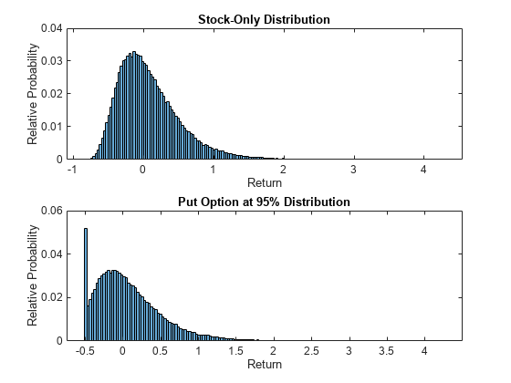
Plot the distribution of the returns for the stock-only strategy and the put option at the 95% strategy. Notice that the returns are not normally distributed. For a mean-variance portfolio, a lack of symmetry in the plotted returns usually indicates poor mean-variance portfolio performance since variance, as a risk measure, is not sensitive to skewed distributions.
% Create histogram
figure;

% Stock only
subplot(2,1,1);
histogram(AssetScenarios(:,1),'Normalization','probability')
title('Stock-Only Distribution')
xlabel('Return')
ylabel('Relative Probability')

% Put option cover
subplot(2,1,2);
histogram(AssetScenarios(:,2),'Normalization','probability')
title('Put Option at 95% Distribution')
xlabel('Return')
ylabel('Relative Probability')
CVaR Efficient Frontier
Create a PortfolioCVaR object using the AssetScenarios from the simulation.
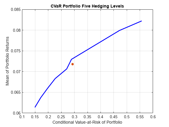
p = PortfolioCVaR('Name','CVaR Portfolio Five Hedging Levels',...
   'AssetList',{'Stock','Hedge50','Hedge75','Hedge90','Hedge95'},...
   'Scenarios', AssetScenarios, 'LowerBound', 0, ...
   'Budget', 1, 'ProbabilityLevel', 0.95);

% Estimate the efficient frontier to obtain portfolio weights
pwgt = estimateFrontier(p);

% Plot the efficient frontier
figure;
plotFrontier(p, pwgt);

CVaR and Mean-Variance Efficient Frontier Comparison
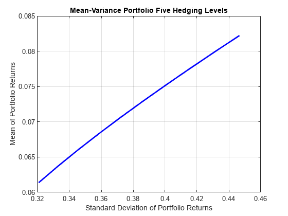
Create the Portfolio object. Use AssetScenarios from the simulation to estimate the assets moments. Notice that, unlike for the PortfolioCVaR object, only an estimate of the assets moments is required to fully specify a mean-variance portfolio.
pmv = Portfolio('Name','Mean-Variance Portfolio Five Hedging Levels',...
   'AssetList',{'Stock','Hedge50','Hedge75','Hedge90','Hedge95'});
pmv = estimateAssetMoments(pmv, AssetScenarios);
pmv = setDefaultConstraints(pmv);

% Estimate the efficient frontier to obtain portfolio weights
pwgtmv = estimateFrontier(pmv);

% Plot the efficient frontier
figure;
plotFrontier(pmv, pwgtmv);
Select a target return. In this case, the target return is the midpoint return on the CVaR portfolio efficient frontier.
% Achievable levels of return
pretlimits = estimatePortReturn(p, estimateFrontierLimits(p));
TargetRet = mean(pretlimits); % Target half way up the frontier
Plot the efficient CVaR portfolio for the return TargetRet on the CVaR efficient frontier.
% Obtain risk level at target return
pwgtTarget = estimateFrontierByReturn(p,TargetRet); % CVaR efficient portfolio
priskTarget = estimatePortRisk(p,pwgtTarget);

% Plot point onto CVaR efficient frontier
figure;
plotFrontier(p,pwgt);
hold on
scatter(priskTarget,TargetRet,[],'filled');
hold off
Plot the efficient CVaR portfolio for the return TargetRet on the mean-variance efficient frontier. Notice that the efficient CVaR portfolio is below the mean-variance efficient frontier.
% Obtain the variance for the efficient CVaR portfolio
pmvretTarget = estimatePortReturn(pmv,pwgtTarget); % Should be TargetRet
pmvriskTarget = estimatePortRisk(pmv,pwgtTarget);  % Risk proxy is variance

% Plot efficient CVaR portfolio onto mean-variance frontier
figure;
plotFrontier(pmv,pwgtmv);
hold on
scatter(pmvriskTarget,pmvretTarget,[],'filled');
hold off
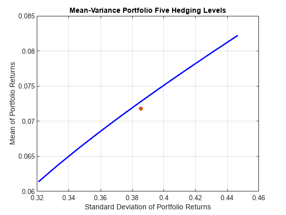
Plot the efficient mean-variance portfolio for the return TargetRet on the CVaR efficient frontier. Notice that the efficient mean-variance portfolio is below the CVaR efficient frontier.
% Obtain the mean-variance efficient portfolio at target return
pwgtmvTarget = estimateFrontierByReturn(pmv,TargetRet);

% Obtain the CVaR risk for the mean-variance efficient portfolio
pretTargetCVaR = estimatePortReturn(p,pwgtmvTarget); % Should be TargetRet
priskTargetCVaR = estimatePortRisk(p,pwgtmvTarget);  % Risk proxy is CVaR

% Plot mean-variance efficient portfolio onto the CVaR frontier
figure;
plotFrontier(p,pwgt);
hold on
scatter(priskTargetCVaR,pretTargetCVaR,[],'filled');
hold off
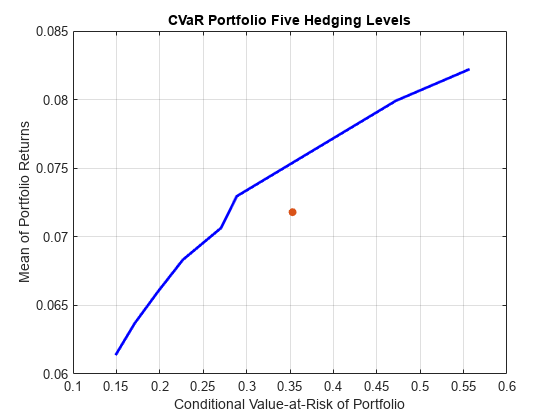
Since mean-variance and CVaR are two different risk measures, this example illustrates that the efficient portfolio for one type of risk measure is not efficient for the other.
CVaR and Mean-Variance Portfolio Weights Comparison
Examine the portfolio weights of the portfolios that make up each efficient frontier to obtain a more detailed comparison between the mean-variance and CVaR efficient frontiers.
Plot the weights associated with the mean-variance portfolio efficient frontier.
% Plot the mean-variance portfolio weights
figure;
area(pwgtmv');
legend(pmv.AssetList);
axis([1 10 0 1])
title('Mean-Variance Portfolio Weights Five Hedging Levels');
xlabel('Portfolios from Minimum(1) to Maximum(10) Return');
ylabel('Contribution of each Asset');
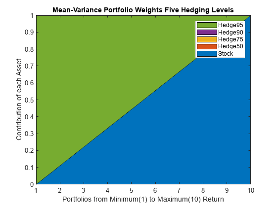
The weights associated with the mean-variance portfolios on the efficient frontier use only two strategies, 'Stock' and 'Hedge95'. This behavior is an effect of the correlations among the five assets in the portfolio. Because the correlations between the assets are close to 1, the standard deviation of the portfolio is almost a linear combination of the standard deviation of the assets. Hence, because assets with larger returns are associated with assets with larger variance, a linear combination of only the assets with the smallest and largest returns is observed in the efficient frontier.
Plot the weights associated with the CVaR portfolio efficient frontier.
% Plot the CVaR portfolio weights
figure;
area(pwgt');
legend(p.AssetList);
axis([1 10 0 1])
title('CVaR Portfolio Weights Five Hedging Levels');
xlabel('Portfolios from Minimum(1) to Maximum(10) Return');
ylabel('Contribution of each Asset');
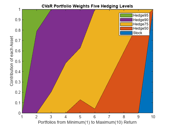
For both types of portfolios, mean-variance and CVaR, the portfolio with the maximum expected return is the one that allocates all the weight to the stock-only strategy. This makes sense because no put options are acquired, which translates into larger returns. Also, the portfolio with minimum variance is the same for both risk measures. This portfolio is the one that allocates everything to 'Hedge95' because that strategy limits the possible losses the most. The real differences between the two types of portfolios are observed for the return levels between the minimum and maximum. There, in contrast to the efficient portfolios obtained using variance as the measure of risk, the weights of the CVaR portfolios range among all five possible strategies.
See Also
PortfolioCVaR | getScenarios | setScenarios | estimateScenarioMoments | simulateNormalScenariosByMoments | simulateNormalScenariosByData | setCosts | checkFeasibility
Topics
- Troubleshooting CVaR Portfolio Optimization Results
- Creating the PortfolioCVaR Object
- Working with CVaR Portfolio Constraints Using Defaults
- Asset Returns and Scenarios Using PortfolioCVaR Object
- Estimate Efficient Portfolios for Entire Frontier for PortfolioCVaR Object
- Estimate Efficient Frontiers for PortfolioCVaR Object
- Compute Maximum Reward-to-Risk Ratio for CVaR Portfolio
- PortfolioCVaR Object
- Portfolio Optimization Theory
- PortfolioCVaR Object Workflow