Compare Hodrick-Prescott Filter Formulations

This example compares two formulations of the Hodrick-Prescott filter: the closed-form solution of the programming problem in [2] and its state-space formulation, with a focus on how each formulation addresses missing observations.

Original Formulation of Hodrick-Prescott Filter

Hodrick and Prescott [1] propose a method for the decomposition of macroeconomic time series ${\mathit{y}}_{\mathit{t}}$ into a trend component ${\tau }_{\mathit{t}}$ and a cyclical component ${\mathit{c}}_{\mathit{t}}$ such that ${\mathit{y}}_{\mathit{t}}={\tau }_{\mathit{t}}+{\mathit{c}}_{\mathit{t}}$. Their trend solved the programming problem

$\underset{{\tau }_{\mathit{t}}}{\min }\left\{{\sum }_{\mathit{t}=1}^{\mathit{T}}{\left({\mathit{y}}_{\mathit{t}}-{\tau }_{\mathit{t}}\right)}^2+\lambda {\sum }_{\mathit{t}=2}^{\mathit{T}-1}{\left[\left({\tau }_{\mathit{t}+1}-{\tau }_{\mathit{t}}\right)-\left({\tau }_{\mathit{t}}-{\tau }_{\mathit{t}-1}\right)\right]}^2\right\}$,

where $\mathit{T}$is the sample size and $\lambda$ is an adjustable smoothing parameter.

Hodrick [2] provides an exact closed-form solution to the linear first-order conditions of the programming problem. The Econometrics Toolbox™ hpfilter function implements this solution. Because the solution is expressed in terms of matrix operations on ${\mathit{y}}_{\mathit{t}}$, hpfilter, and the filter functions bkfilter, cffilter, and hfilter, require that the input series contain complete data (no missing values).

Hodrick [2] states, "While Hodrick and Prescott [1] were aware of this direct solution, it involves inversion of a $\left(\mathit{T}+2\right)$ x $\left(\mathit{T}+2\right)$ matrix, which they viewed as potentially problematic given the memory capacity of computers in 1978." However, the MATLAB® function mldivide performs the required matrix algebra accurately and efficiently.

Hodrick and Prescott [1] solve the programming problem by viewing the programming problem as a state-space model and applying the Kalman filter [3]. The state-space representation requires assumptions on the distributions of the components ${\tau }_{\mathit{t}}$ and ${\mathit{c}}_{\mathit{t}}$. Hodrick [2] states, "It is important to note that Hodrick and Prescott [1] explicitly argued that this specific probability model was false, and they were sensitive to the fact that the results could depend on the choice of $\lambda$." However, the resulting state-space representation allowed them to introduce prior information on the specific macroeconomic series under consideration, and so to choose an empirical value of $\lambda$. Also, the Kalman filter can return forecasted and smoothed output on input series with incomplete data.

State-Space Representation of Hodrick-Prescott Filter

Hodrick and Prescott [1] introduce the model by stating: "The following probability model is useful for bringing to bear prior knowledge in the selection of the smoothing parameter $\lambda$. If the cyclical components and the second difference of the growth components were identically and independently distributed normal variables with means zero and variances ${\sigma }_1^2$ and ${\sigma }_2^2$ (which they are not), the conditional expectation of the ${\tau }_{\mathit{t}}$, given the observations, would be the solution to programming problem when $\sqrt{\lambda }={\sigma }_1/{\sigma }_2$."

With these assumptions and $\sqrt{\lambda }={\sigma }_1/{\sigma }_2$, the programming problem is

$\underset{{\tau }_{\mathit{t}}}{\min }\left\{{\sum }_{\mathit{t}=1}^{\mathit{T}}{\left({\mathit{y}}_{\mathit{t}}-{\tau }_{\mathit{t}}\right)}^2+\left(\frac{{\sigma }_1^2}{{\sigma }_2^2}\right){\sum }_{\mathit{t}=2}^{\mathit{T}-1}{\left[\left({\tau }_{\mathit{t}+1}-{\tau }_{\mathit{t}}\right)-\left({\tau }_{\mathit{t}}-{\tau }_{\mathit{t}-1}\right)\right]}^2\right\}$.

Combining terms and factoring out ${\sigma }_1^2$, the programming problem is

$\underset{{\tau }_{\mathit{t}}}{\min }\left\{\left(\frac{1}{{\sigma }_1^2}\right){\sum }_{\mathit{t}=1}^{\mathit{T}}{\left({\mathit{y}}_{\mathit{t}}-{\tau }_{\mathit{t}}\right)}^2+\left(\frac{1}{{\sigma }_2^2}\right){\sum }_{\mathit{t}=2}^{\mathit{T}-1}{\left({\tau }_{\mathit{t}+1}-2{\tau }_{\mathit{t}}+{\tau }_{\mathit{t}-1}\right)}^2\right\}$.

Obtain the state-space representation of the programming problem, proposed by Hodrick and Prescott [1], by viewing the two summands as random variables:

• Measurement Equation — Set the cyclical component to a normal variable with variance ${{\sigma }_1^2=\sigma }^2$: ${{\mathit{c}}_{\mathit{t}}=\mathit{y}}_{\mathit{t}}-{\tau }_{\mathit{t}}={\epsilon }_{\mathit{t}}$, or ${\mathit{y}}_{\mathit{t}}={\tau }_{\mathit{t}}+{\epsilon }_{\mathit{t}}$ with ${\epsilon }_{\mathit{t}}\sim \mathit{N}\left(0,{\sigma }^2\right)$.

• State Equation — Set the second difference of the growth (trend) component to a normal variable with variance ${\sigma }_2^2={\sigma }^2/\lambda$: ${\tau }_{\mathit{t}+1}-{2\tau }_{\mathit{t}}+{\tau }_{\mathit{t}-1}={\mathit{u}}_{\mathit{t}}$, or the following system of equations, with ${\mathit{u}}_{\mathit{t}}\sim \mathit{N}\left(0,{\sigma }^2/\lambda \right)$.

$$\begin{array}{l}{\tau }_t=2{\tau }_{t-1}-{\nu }_{t-1}+u_t\\ {\nu }_t={\tau }_{t-1}.\end{array}$$

In matrix form, the model is

$$\begin{array}{l}\left[\begin{array}{l}{\tau }_t\\ {\nu }_t\end{array}\right]=\left[\begin{array}{cc}2& -1\\ 1& 0\end{array}\right]\left[\begin{array}{l}{\tau }_{t-1}\\ {\nu }_{t-1}\end{array}\right]+\left[\begin{array}{l}\sigma /\sqrt{\lambda }\\ 0\end{array}\right]u_t\\ y_t={\tau }_t+{\epsilon }_t.\end{array}$$

Create a state-space model of the programming problem by using the ssm function. Set $\sigma =5$ and $\lambda =1600$, as proposed in [1] for quarterly data.

sigma = 5;
lambda = 1600;

A = [2 -1; 1 0];
B = [sigma/sqrt(lambda);0];
C = [1 0];
D = sigma;

SSMdlHP = ssm(A,B,C,D);

disp(SSMdlHP)

State-space model type: ssm

State vector length: 2
Observation vector length: 1
State disturbance vector length: 1
Observation innovation vector length: 1
Sample size supported by model: Unlimited

State variables: x1, x2,...
State disturbances: u1, u2,...
Observation series: y1, y2,...
Observation innovations: e1, e2,...

State equations:
x1(t) = (2)x1(t-1) - x2(t-1) + (0.12)u1(t)
x2(t) = x1(t-1)

Observation equation:
y1(t) = x1(t) + (5)e1(t)

Initial state distribution:

Initial state means
 x1  x2 
  0   0 

Initial state covariance matrix
     x1     x2    
 x1  1e+07  0     
 x2  0      1e+07 

State types
    x1       x2   
 Diffuse  Diffuse 

The software analyzes the transition matrix A. Because its eigenvalues are on the unit circle, a stationary distribution does not exist. Therefore, the default state types are diffuse, as discussed in [1].

Compare Formulations

Compare the state-space model with the closed form solution implemented by hpfilter. Consider the complete quarterly data on US gross domestic product (GDP).

load Data_GDP
GDP = DataTimeTable.GDP;   
tGDP = DataTimeTable.Time; 

Compute the trend component by passing the state-space model and data to the smooth function, and then extract the first variable from the output. smooth applies the Kalman filter to smooth the states; the first variable in the output is the unlagged smoothed trend estimate.

States = smooth(SSMdlHP,GDP); 
ssTrend = States(:,1); 

Compute the trend component by passing the data and smoothing parameter to hpfilter. The result is the closed-form solution of the programming problem.

hpTrend = hpfilter(GDP,Smoothing=lambda); % Apply closed form

Plot of the two trend estimates and their difference.

figure
hold on
plot(tGDP,GDP,"b-",LineWidth=2)
plot(tGDP,ssTrend,"r-",LineWidth=2)
plot(tGDP,hpTrend,"g--",LineWidth=2)
ylabel("Billions of Dollars")
title("Gross Domestic Product")
legend(["GDP" "ssTrend" "hpTrend"],Location="northwest")
grid on
hold off

figure
plot(hpTrend-ssTrend,LineWidth=2)
xlabel("Kalman Filter Iteration")
ylabel("Difference")
title("State-Space vs. Closed-Form Solution")
grid on

With the exception of small differences during the initialization period of the Kalman filter, the trend estimates are virtually indistinguishable.

In most models, initial conditions have limited impact on the Kalman filter. Because the differences are on the order of ${10}^{-4}$ are compared to GDP data on the order of ${10}^3$, the transient differences have no economic significance. If other initial conditions are specified, the initialization changes slightly, but the impact decreases over time.

Address Missing Values

In addition to the ability of the Kalman filter to estimate parameters in a state-space model, it processes missing values by using a combination of forecasting and smoothing.

Introduce 10 missing values in the middle of the GDP data.

GDP0 = GDP;
GDP0(101:110) = NaN; 
dataLength = length(GDP0)

dataLength = 
234

Pass the state-space model and incomplete data to smooth. Despite the missing observations, the Kalman filter returns a complete trend the same size as the incomplete input data.

States0 = smooth(SSMdlHP,GDP0);
ssTrend0 = States0(:,1);
ssTrend0Length = length(ssTrend0)

ssTrend0Length = 
234

By contrast, hpfilter removes missing values through listwise deletion, producing a trend on the complete, but compressed, time base.

hpTrend0 = hpfilter(GDP0,Smoothing=lambda);
hpTrend0Length = length(hpTrend0)

hpTrend0Length = 
224

The behavior of hpfilter is consistent with most functions in Econometrics Toolbox that implement matrix algorithms for efficiency. In a closed-form solution, matrix algebra proliferates, rather than imputes, missing values.

Government sources offer complete data on the majority of economic indicators. However, if your data contains missing values, employ imputation methods in a preprocessing step before you use hpfilter. For small gaps in the data, interpolation methods, such as those implemented by the MATLAB function interp1, are often sufficient. (See [5] for a methods specific to Hodrick-Prescott filtering.) When input data contains larger gaps, accurate imputation requires a model of the data. If the model can be given a state-space representation, you can impute missing data using the Kalman filter. For example, the GDP data is notoriously difficult to model (see, for example, [4]), but you can approximately describe it by using an ARIMA model, which has a state-space representation.

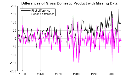
Apply the second difference of the incomplete GDP data , and plot the result. The result appears to be roughly stationary.

D1GDP0 = diff(GDP0);    
D2GDP0 = diff(D1GDP0);  

figure
hold on
plot(tGDP(2:end),D1GDP0,"k-")
plot(tGDP(3:end),D2GDP0,"m-")
title("Differences of Gross Domestic Product with Missing Data")
legend(["First difference" "Second difference"],Location="northwest")
grid on
hold off

Confirm the stationarity of the second difference by conducting paired unit root and stationarity tests using the i10test function.

[h,pValue] = i10test(D2GDP0,VarNames="D2GDP");

Test Results

        I(1)    I(0)    
======================
D2GDP   1       0       
        0.0010  0.1000  
----------------------

The test rejects a unit root (I(1) = 1) using the default augmented Dickey-Fuller test (see adftest), but it fails to reject stationarity (I(0) = 0) using the default KPSS test (see kpsstest).

Thus, for preprocessing purposes, you can describe the GDP as a simple ARIMA(1,2,1) model, which is an ARMA(1,1) model when you apply the second difference to the response: ${\mathit{y}}_{\mathit{t}}=\phi {\mathit{y}}_{\mathit{t}-1}+{\epsilon }_{\mathit{t}}+\theta {\epsilon }_{\mathit{t}-1}$ with ${\epsilon }_{\mathit{t}}\sim \mathit{N}\left(0,{\sigma }^2\right)$.

The ARMA model has the state-space representation represented in the paramMap function. Because the parameter $\sigma$ determines both the A and B matrices, use a function handle to map the parameters $\phi$, $\theta$, and $\sigma$ to the state-space model matrices.

SSMdlGDP = ssm(@paramMap);

function [A,B,C,D] = paramMap(params)
    phi = params(1);
    theta = params(2);
    sigma = params(3);
    A = [phi theta*sigma; 0 0];
    B = [sigma; 1];
    C = [1 0];
    D = [];
end

Fit the model to the incomplete data in the second difference. Specify arbitrarily chosen initial parameter values for estimation.

params0 = [0.5; 0.5; 0.1];
EstMdl = estimate(SSMdlGDP,D2GDP0,params0,Display="off",Univariate=true);

Impute the missing data using the Kalman filter by passing the fitted model and incomplete data to smooth.

StatesD20 = smooth(EstMdl,D2GDP0);
D2GDP0Imputed = StatesD20(99:110,1);

Recover the levels in the GDP by integrating the differences.

D1GDP0Imputed = cumsum([D1GDP0(99); D2GDP0Imputed]); 
GDP0Imputed = cumsum([GDP0(100); D1GDP0Imputed]);

figure
hold on
plot(tGDP(90:120),GDP0(90:120),"b-",LineWidth=2)
plot(tGDP(101:110),GDP(101:110),"bo")
plot(tGDP(101:110),GDP0Imputed(2:11),"b*")
ylabel("Billions of Dollars")
title("Gross Domestic Product with Missing Data")
legend(["GDP" "Missing data" "Imputed data"],Location="northwest")
grid on
hold off

Pass the completed data directly to hpfilter for estimation of the trend on the original time base.

GDP0Filled = GDP0;
GDP0Filled(101:110) = GDP0Imputed(2:11);
hpTrendFilled = hpfilter(GDP0Filled);

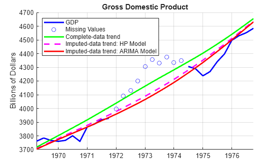
Compare the trends computed by different methods.

figure
hold on
plot(tGDP(90:120),GDP0(90:120),"b-",LineWidth=2)
plot(tGDP(101:110),GDP(101:110),"bo")
plot(tGDP(90:120),hpTrend(90:120),"g-",LineWidth=2)
plot(tGDP(90:120),ssTrend0(90:120),"m--",LineWidth=2)
plot(tGDP(90:120),hpTrendFilled(90:120),"r-",LineWidth=2)
ylabel("Billions of Dollars")
title("Gross Domestic Product")
legend(["GDP" "Missing Values" ...
        "Complete-data trend" ...
        "Imputed-data trend: HP Model" ...
        "Imputed-data trend: ARIMA Model"],Location="northwest")
grid on
hold off

In this case, the Hodrick-Prescott model slightly out-performs the ARIMA(1,2,1) model by producing a trend closer to the complete data trend.

References

[1] Hodrick, Robert J., and Edward C. Prescott. "Postwar U.S. Business Cycles: An Empirical Investigation." Journal of Money, Credit and Banking 29, no. 1 (February 1997): 1–16. https://doi.org/10.2307/2953682.

[2] Hodrick, Robert J. "An Exploration of Trend-Cycle Decomposition Methodologies in Simulated Data." National Bureau of Economic Research Working Paper No. w26750. Social Science Research Network (February 2020). https://papers.ssrn.com/abstract=3539317.

[3] Kalman, Rudolf E. "A New Approach to Linear Filtering and Prediction Problems." Journal of Basic Engineering 82, no. 1 (March 1960): 35–45. https://doi.org/10.1115/1.3662552.

[4] Nelson, Charles R., and Charles R. Plosser. "Trends and Random Walks in Macroeconomic Time Series." Journal of Monetary Economics 10, no. 2 (January 1982): 139–162. https://doi.org/10.1016/0304-3932(82)90012-5.

[5] Schlicht, Ekkehart. "Trend Extraction From Time Series With Missing Observations." Ludwig-Maximilians-Universität München, Volkswirtschaftliche Fakultät, München Munich Discussion Paper 2007-18 (May 2007). https://doi.org/10.5282/ubm/epub.1927.